Topics

Core Topics for the Second Project

• RC and LR circuits
• Op-Amp Circuits
• Introduction to Frequency Response

Project Items

This project primarily gets the students comfortable with measurement and resulting analysis of time-domain (first-order) circuits as well as op-amp circuits. We will work through a few steps to get the desired circuit operation.

(a)

(b)

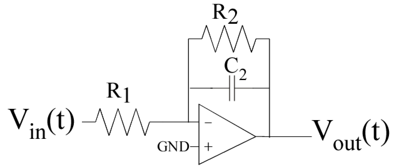
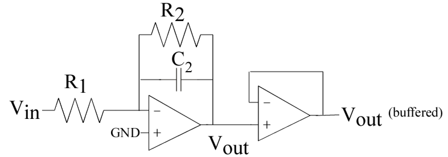
Figure 1: A first-order circuit using an op-amp. (a) Op-Amp based first-order circuit. (b) Using a second Op-Amp in a buffer configuration to buffer the Op-Amp first-order circuit.

The particular components (R and C) that you will use for this project are flexbile, although they need to be explicitly mentioned in your writeup and used throughout your analysis.

The op-amps, or at least approximations of them, are actually physical devices, typically made from transistor circuits. The key is for your op-amp chip to find pins for the positive and negative inputs and output terminals. Remember the circuit requires power supply pins. Either +5V, -5V or +15V, -15V will work.
You need to make sure the pinout you are using for your op-amp.
There are standards, but you need to know which one you are using. Pin 1 is marked by stamp or mark near that pin.

• Low-Frequency Response : Set up the circuit in Fig. 1a without the capacitor element (just the two resistors) such that the magnitude of the gain between input and output is between 1 and 4. Take an voltage sweep and curve fit to show the resulting circuit gain. The input voltage can be swept for this measurement between 0 to 1V, 0.5V to 1.5V, or a similar operating range.
• Buffered Low-Frequency Response : Repeat the above measurement for the buffered circuit in Fig. 1b (again, no capacitor). The Op-amp buffer isolates your circuit output and your instrumentation. An op-amp is configured as a buffer by connecting the - terminal to the output terminal. The + terminal is the input, and the output terminal is the output. Compare the difference of the two measurements when adding this Op-Amp buffer. Explain any other aspects you might notice (e.g. offset). You will want the measurements and curve fits on the same single plot.
• Set up the First-Order Circuit : Set up the First-Order RC circuit in Fig. 1b. You might want to repeat the voltage sweep on this circuit with the capacitor (C₂) to verify everything looks the same as the previous measurements.
• Perform a step response (Fig. 1): This means you have a square wave input and look at the resulting output voltage. Put in an input step between 0.6V and 1.2V. You have a dc voltage of 0.9V. Analytically solve for the RC timeconstant and for V_out response with time, as well as use your experimental data to experimentally measure (curve fit) the RC timeconstant. You will perform a curve fit for the resulting time constant , a curve fit to the exponentially decreasing and exponentially increasing data. Do the two time-constant values agree? You need to include a plot of the measured data with curve fits for the time-constant of the measured data.
• Frequency response (Fig. 1): Use your data aquisition device function, or other means you have available to you, to do a frequency sweep. the device inputs a single frequency and measures the result. Compare your measured frequency response to your expected result.
• Different R and C values: You will change one resistor and change one capacitor value and repeat the above analysis. Both analytically predict the response and measure the time-domain response and frequency response. Compare the analytical values with the devices used. You will want the step response results and time-constant results efficiently plotted in your report. You will want a single plot of the two frequency responses.