Project 1: Numerical ODE Solutions for ML Concepts

This project begins the process of simulating and computing neural network structures. This project enables you to develop your own ODE computing platform.

Your final code that you used for this project should be in a separate file from your writeup.

ODE Solutions

Every class coding example will formulate and numerically solve computation and learning algorithms from an ODE formulation. Types of ODE solvers, order of convergence

Euler Method: Order 1
Runga Kutta (RK) Methods: Order 2 and higher
Predictive RK Methods: e.g. RK45: 4th order RK computation, 5th order estimation for h.
Stiff Differential Equations

ODE routines and computation

MATLAB Code:
[x,y]=ode45( ); Runga-Kutta 4_th order/5_th order predictive model
[x,y]=ode23( ); Runga-Kutta 2_th order/3_th order predictive model
[x,y]=ode15s( ); [x,y]=ode23s( ); Solve stiff differential equations — low order method

Python Code:
odeint( );
solve_ivp( method = 'RK45' )

References:

Texas A&M ODE MATLAB reference: pdf

MATLAB ODE overview: pdf

MATLAB solution of ODEs examples: pdf

Solving ODEs in Python: pdf

Halvorsen on Python ODE solutions: pdf

Order of ODE algorithms

n-order method shows computation within hⁿ⁺¹ of the numerical accuracy.
n-order method error bounds are within the fⁿ⁺¹( ). High derivative (and increasing derivatives, e.g. exp( )) result in wide error bounds (potentially high error) that can lead to a lack of solution stability.

Numerics for Stiff Differential Equations

Roughly 1-bit error every 4 additions.
ODEs have continuous addition of variables (smaller h, proportionally higher error)
Smaller h, more issues with lsb errors.
Longer running sequences result in higher numerical error

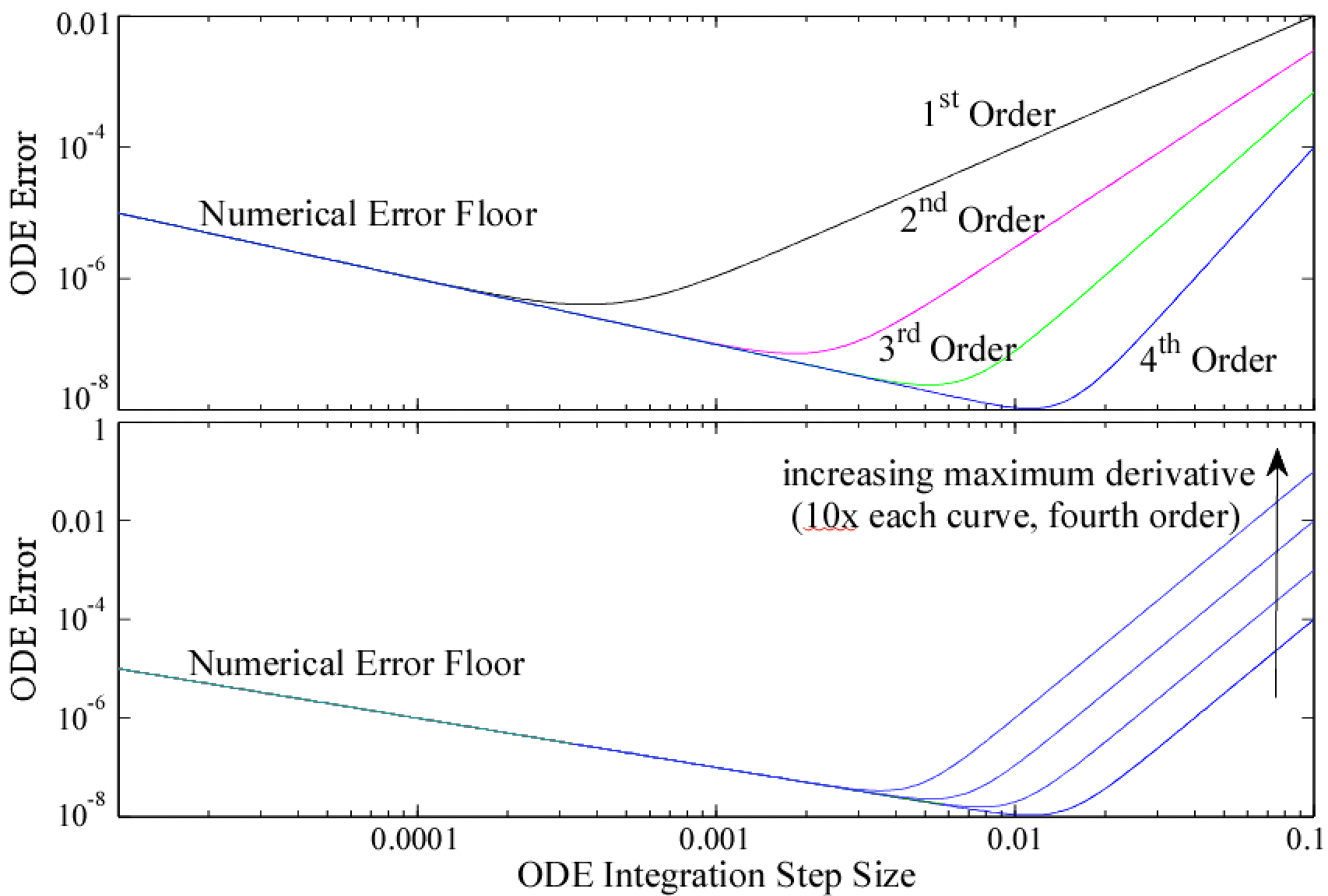
Figure 1: Numerical ODE solution convergence and numerical error as a function of ODE numerical approximation and as a function of numerical derivative estimation.

Numerical Solution of ODE references:

On-line textbook (K. Atkinson, et. al)

Numerical Simulation of Differential Equations

Numerical solution of ODEs is a critical aspect of exploring Neural Network algorithms.

Simulate the following ODE system:

x(t) = cos(2 π f t + θ ), where f = 1kHz, with phase θ
the input dimension of x(t) is 10 or larger with different phases.
τ is 0.2ms
τ w'(t) = y * x (vector) - y² w
y(t) is a single dimension, y(t) = W^T (vector) x(t)`
Simulate this ODE for 5 seconds of physical time.
Show w(t) and y(t)

It is assumed you will be using an ODE solver package that you will be using throughout the semester. Just explaining which package you are using is sufficient. You need to show me the code that you wrote for this simulation (e.g. not the ODE libraries that you used.