Topics
These are the core topics for Unit 2.
These topics are what what would be covered in the exam for Unit 2.
- RC and LR circuits
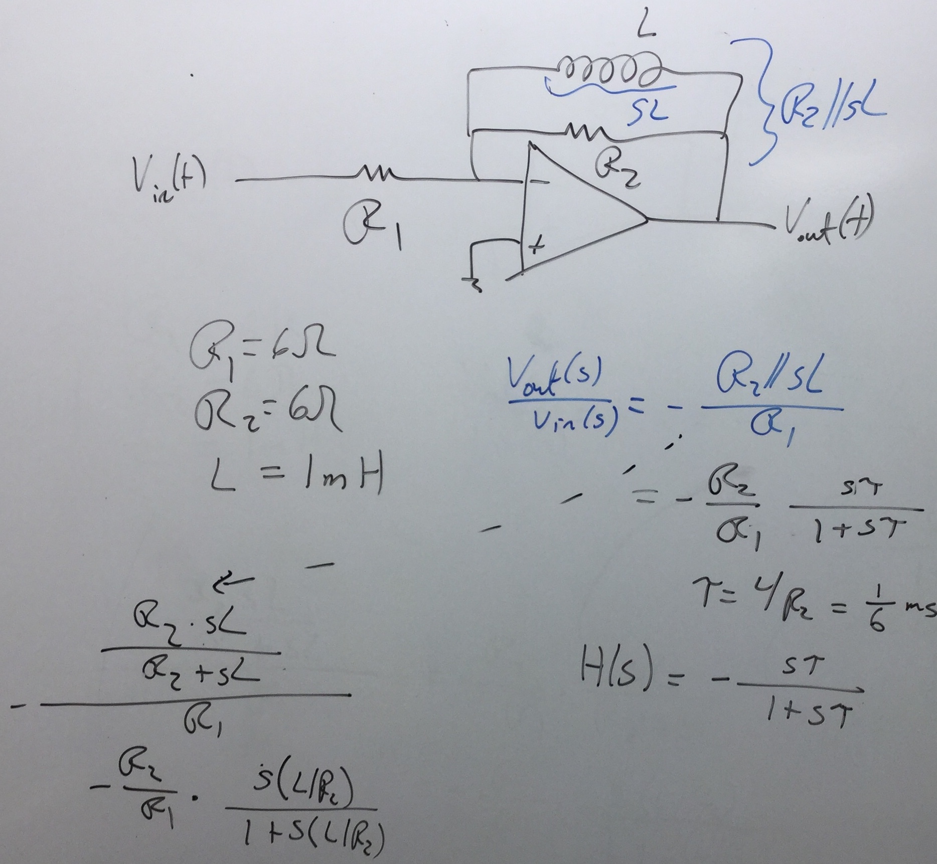
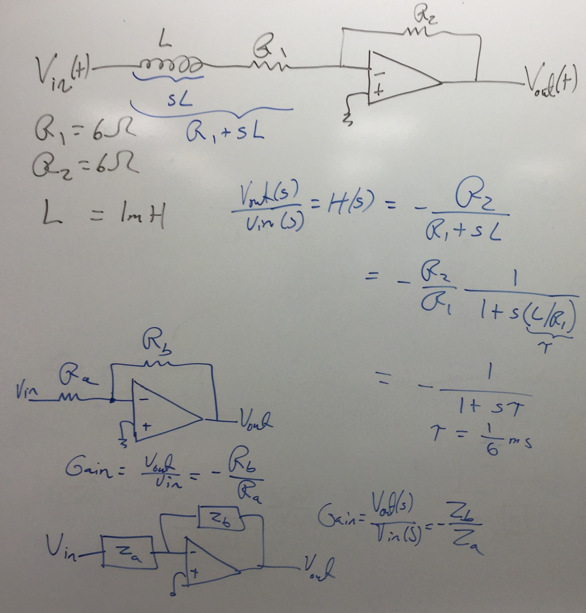
- Op-Amp Circuits
- Laplace Transform solutions of linear circuits
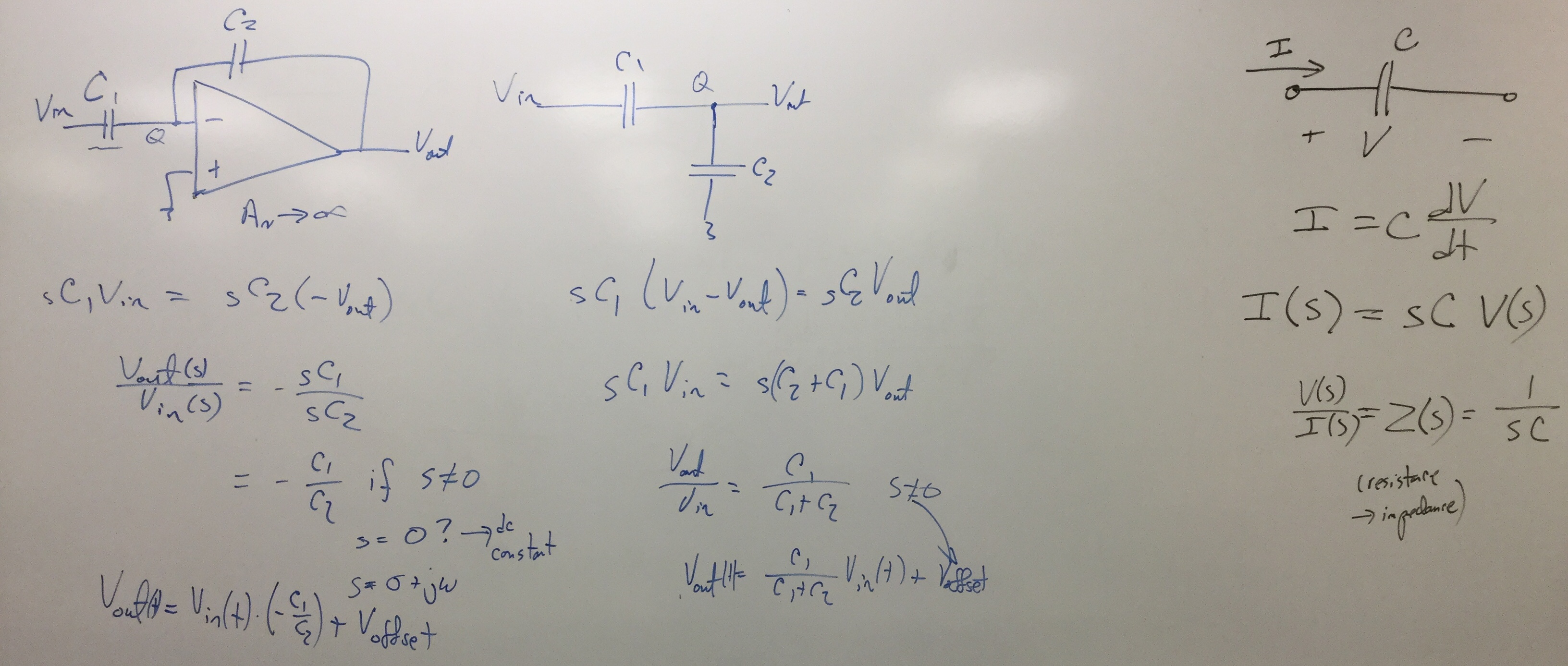
- Using laplace transform representations of capacitors and inductors
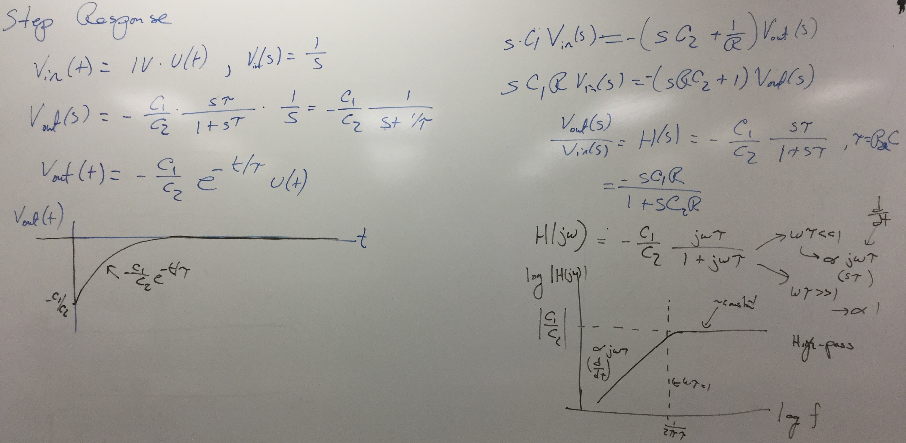
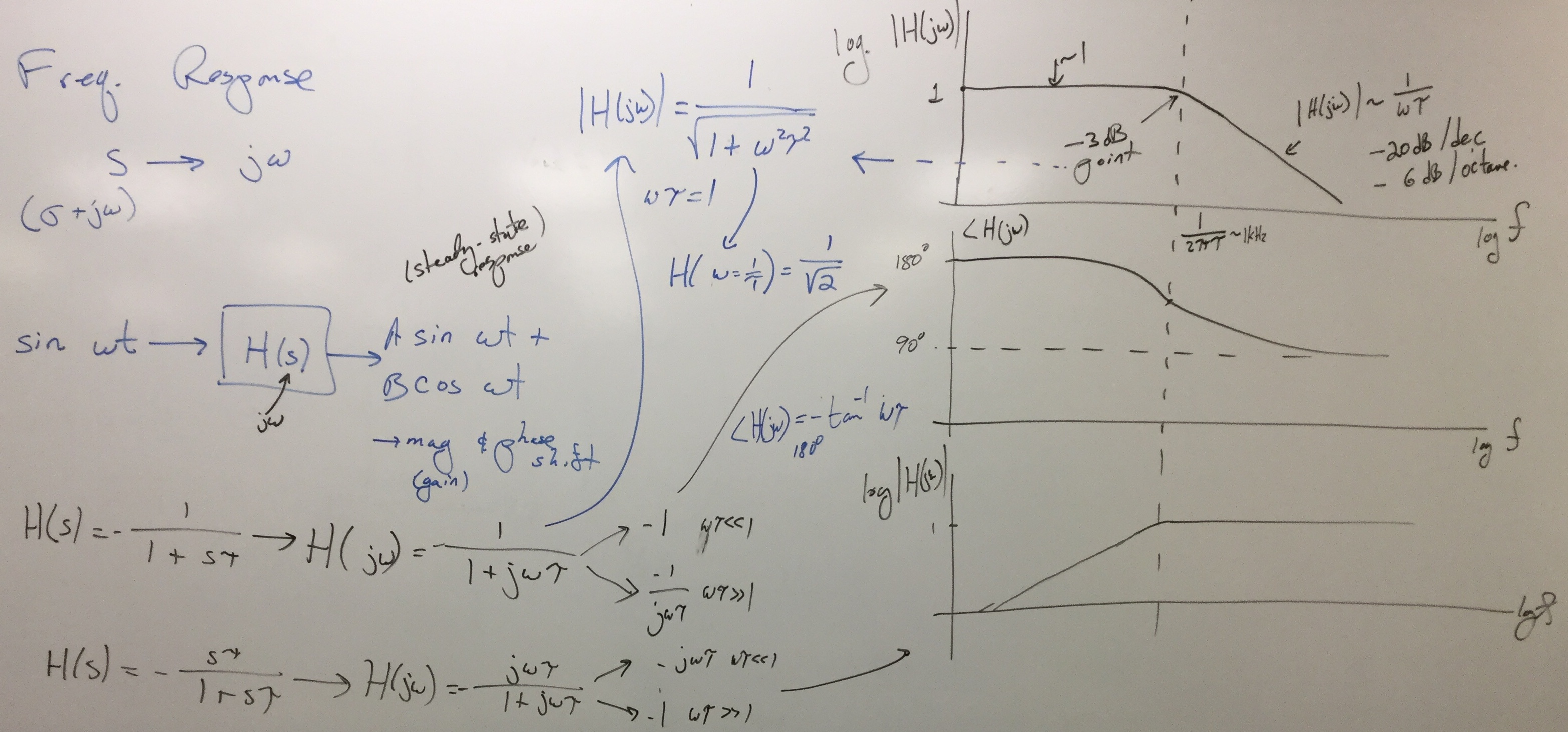
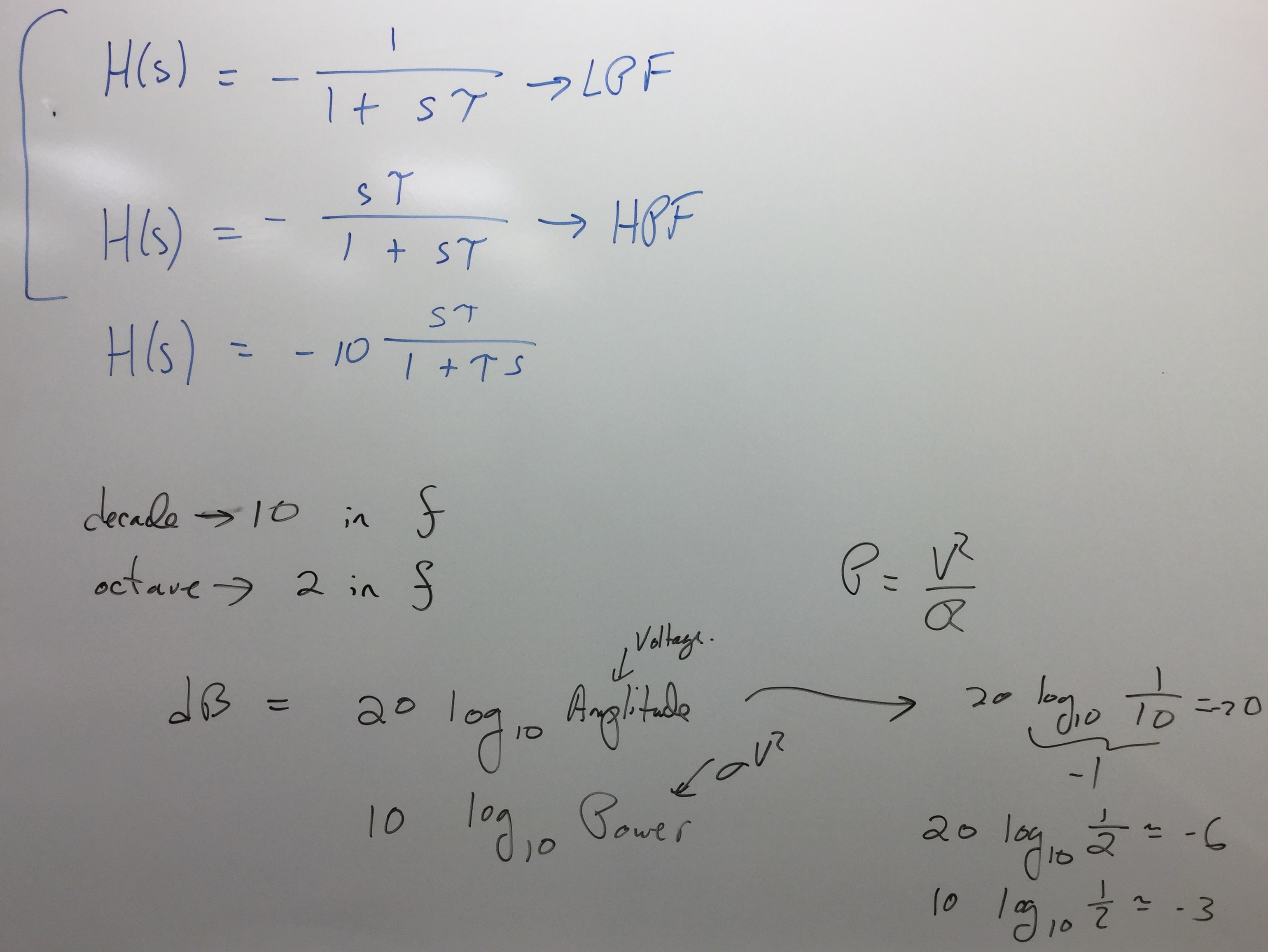
- Introduction to Frequency Response
Class Schedule, Topics, Taped Lectures
The particular taped lectures should be watched before class session.
My photographs of the lecture boards will be posted soon after all lectures are finished.
|
Date
|
Class Topic
|
On-Line Lectures
|
White Boards
| |
Sept 15
|
1st Order Circuits
|
First-order
Dynamics 1,
HPF Dynamics
Thevenin Equivalent RC
Dependent Source
One-Port Equivalent RC
|
1,
2,
3,
4,
5,
6,
7,
8,
| |
Sept 17
|
Op-Amp Resistive Circuits
|
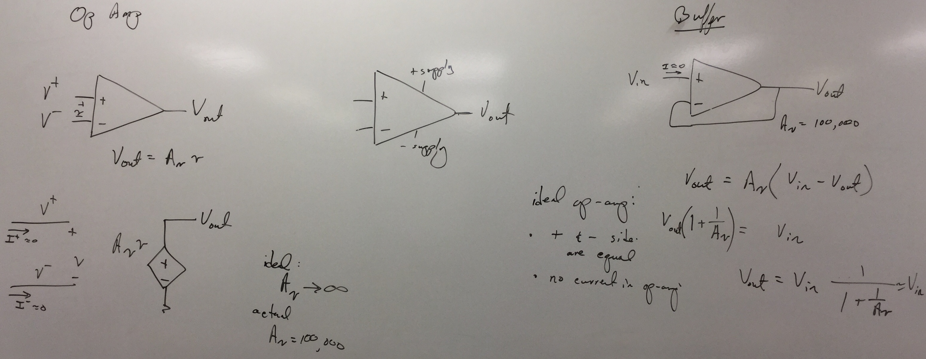
Op-Amp
Intro ,
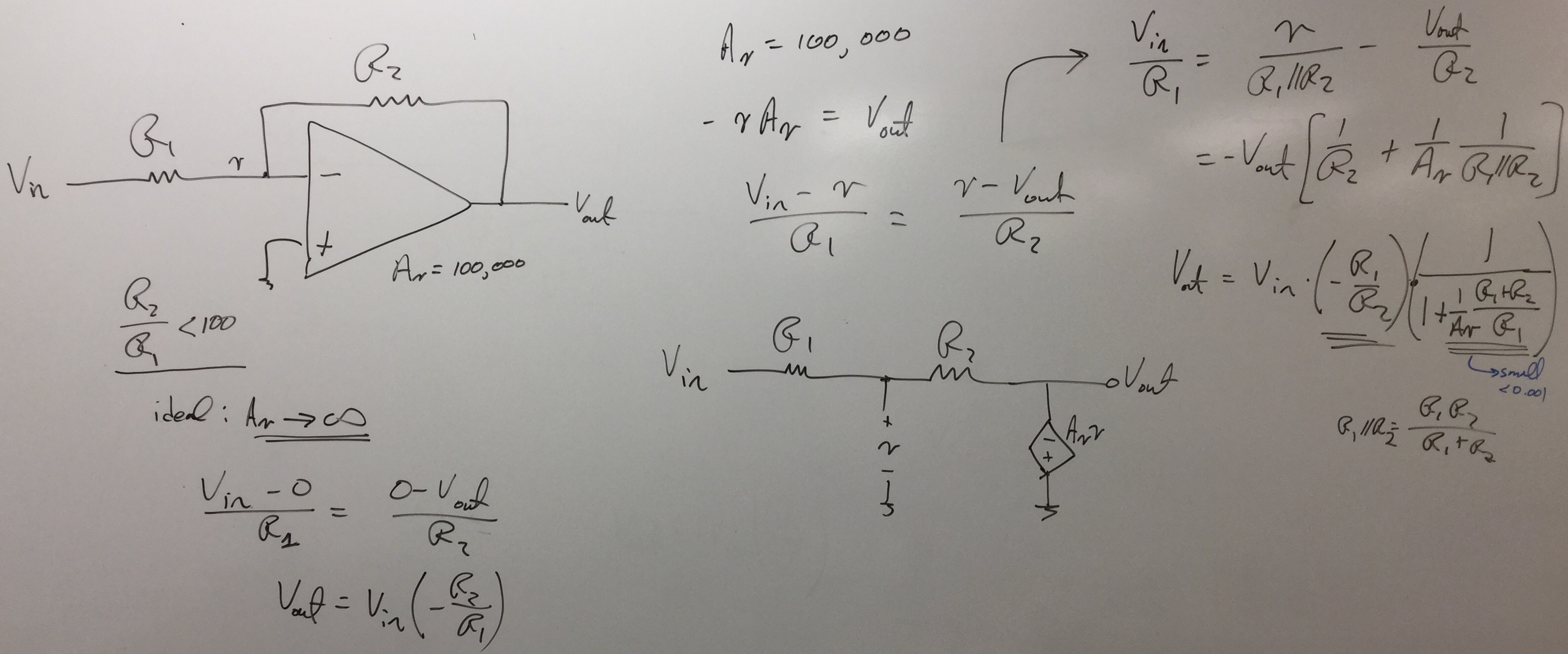
Fund. Circuits ,
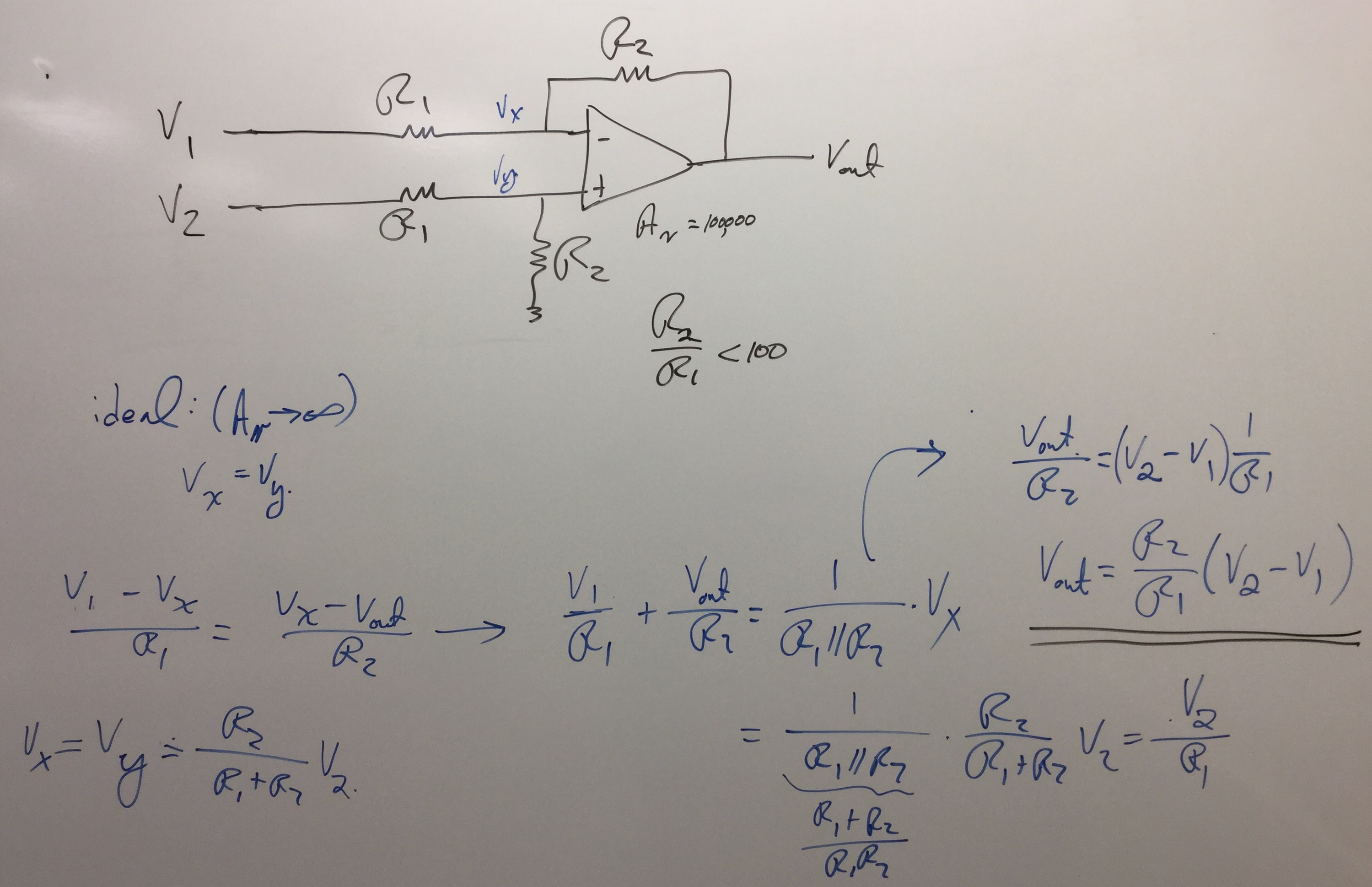
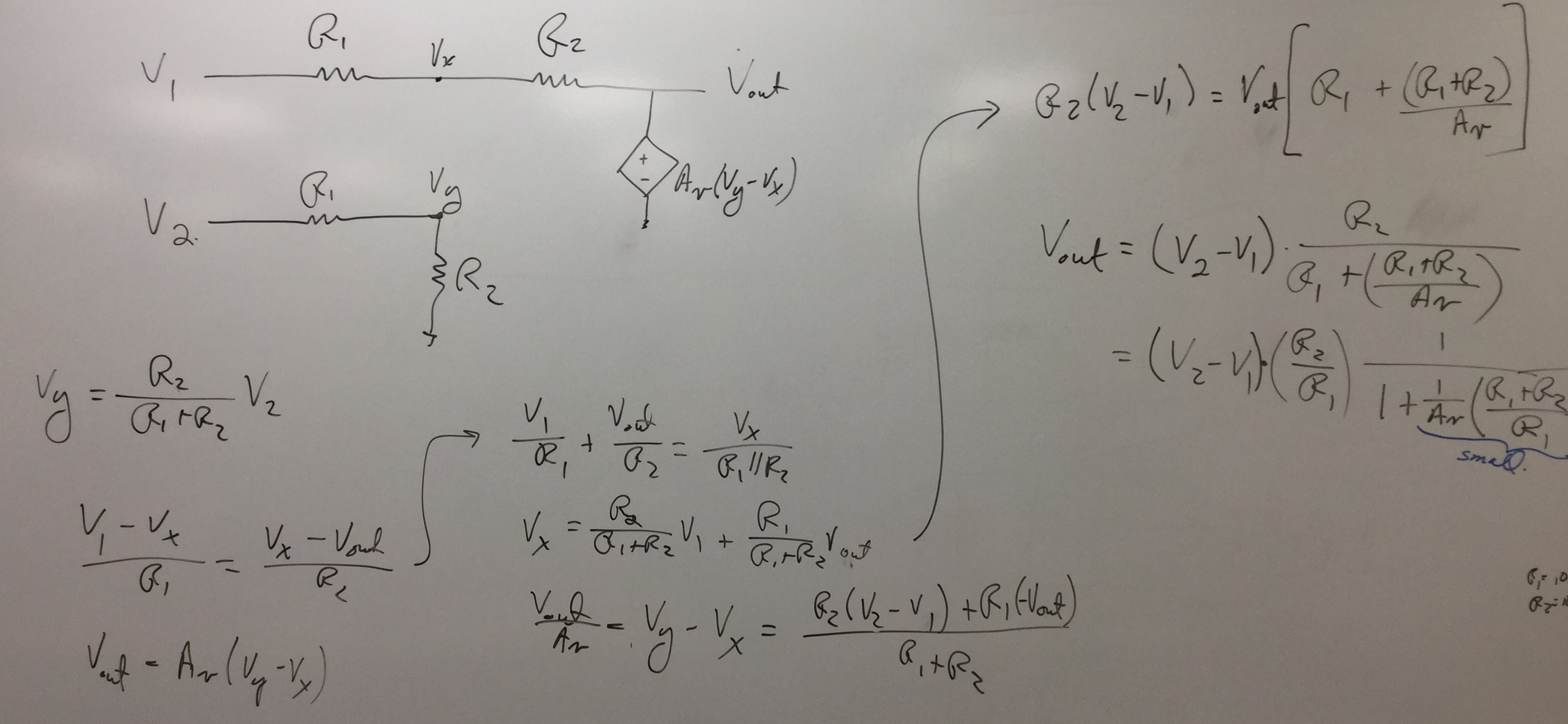
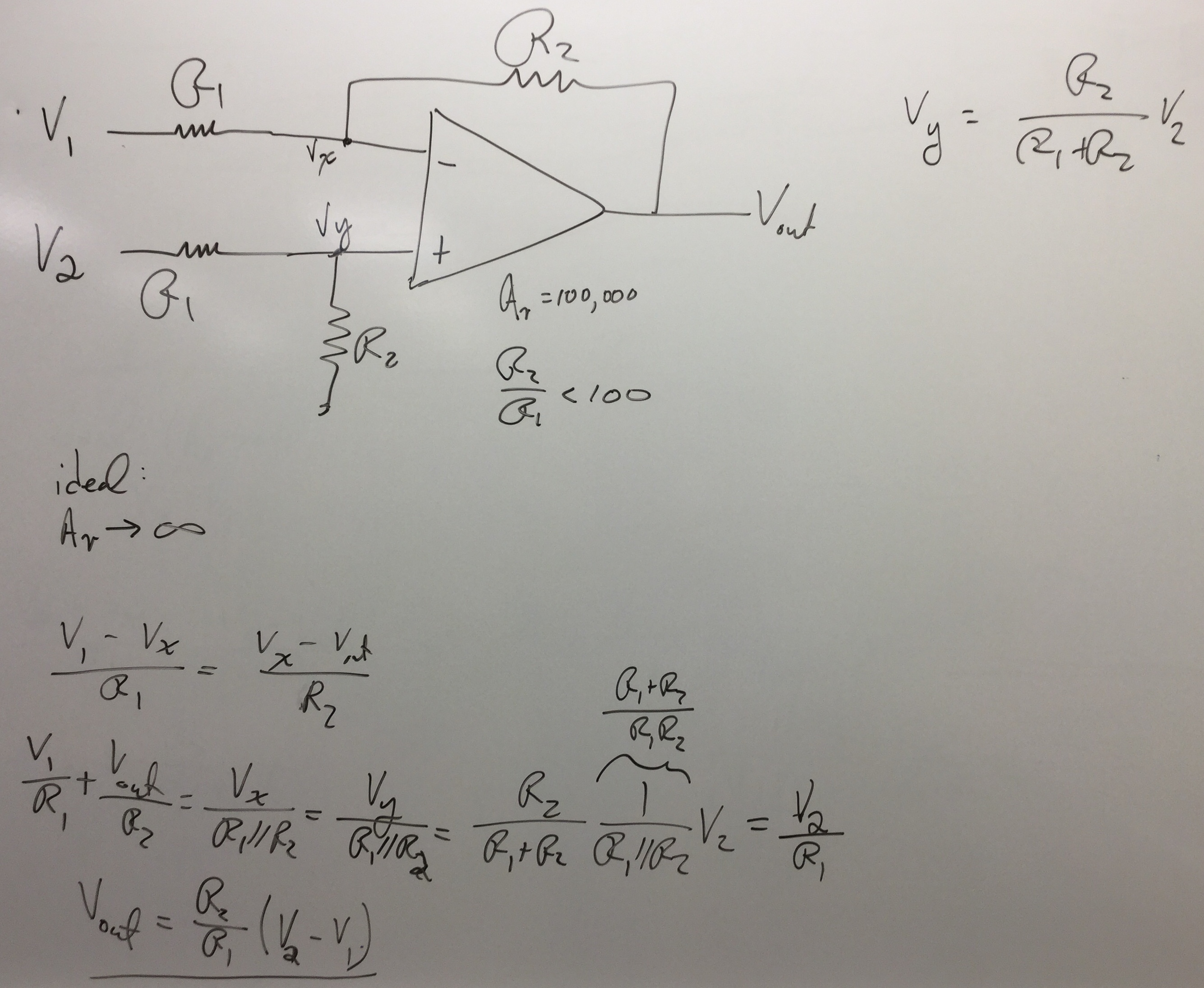
Instrumention ,
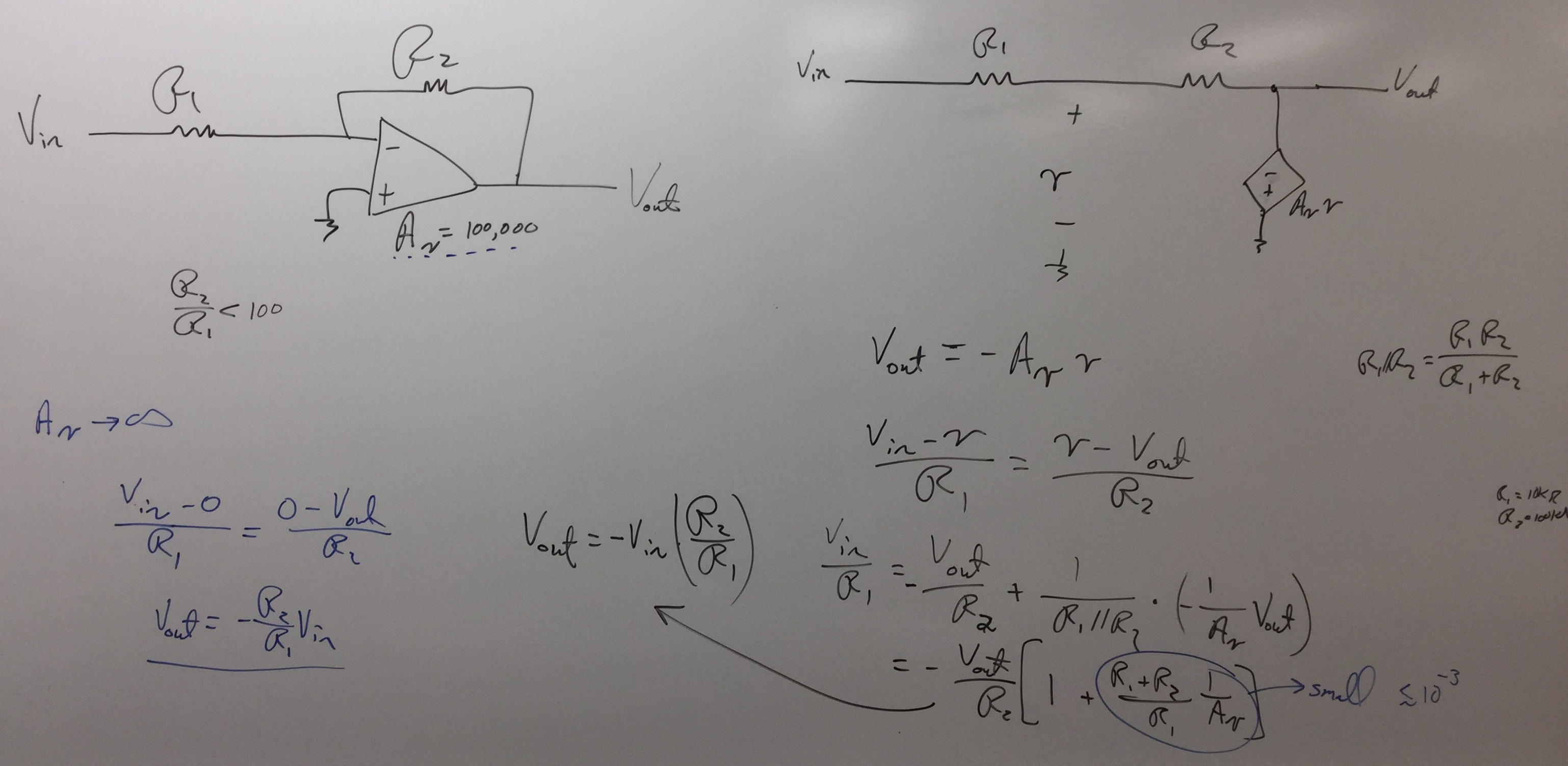
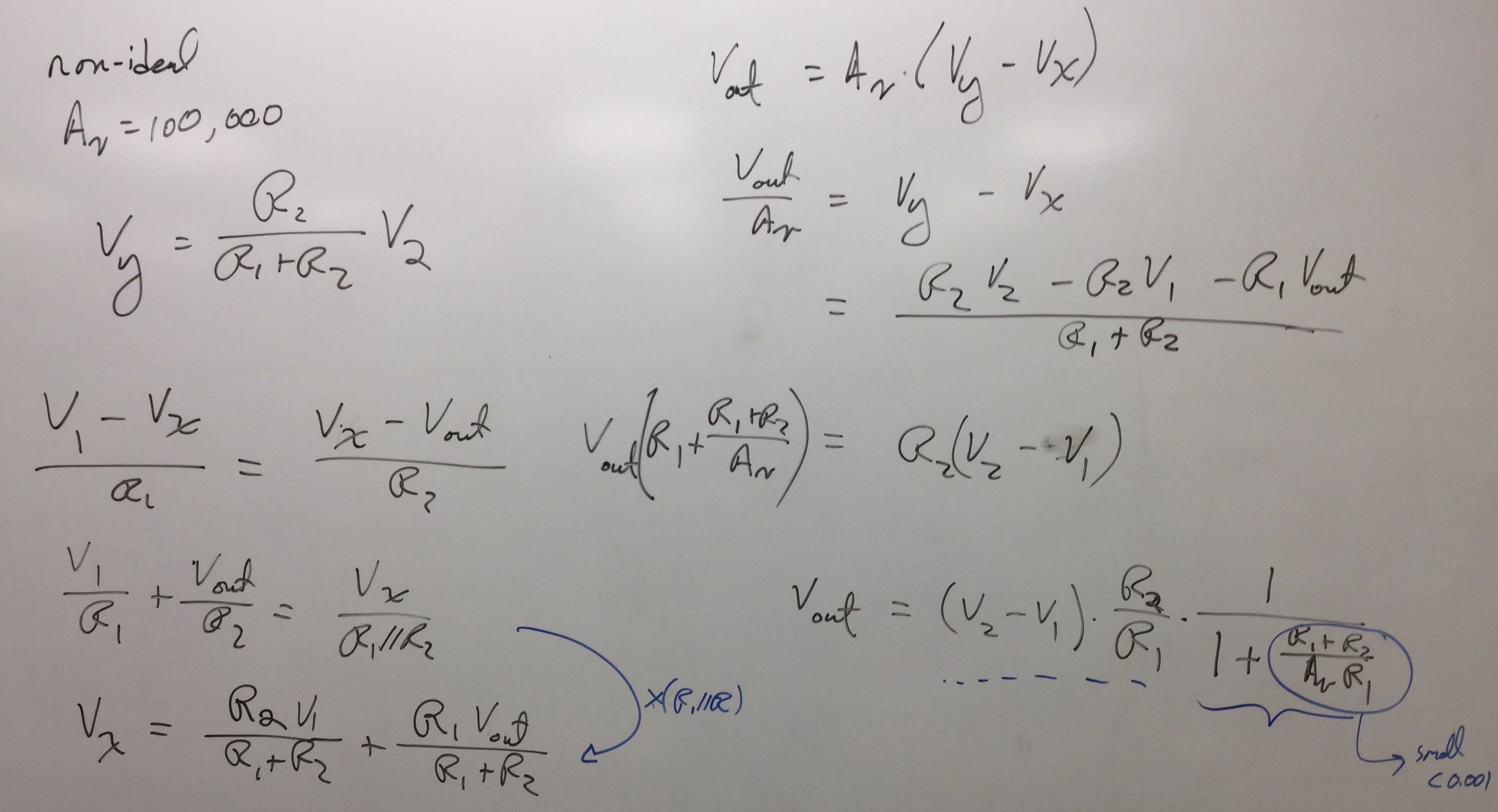
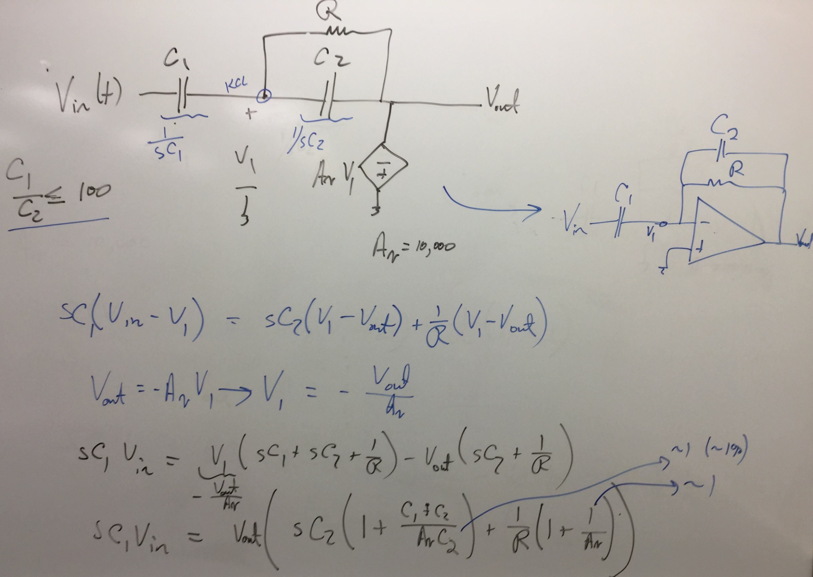
Finite Gain 1,
Finite Gain 2
|
1,
2,
3,
4,
5,
6,
7,
8,
| |
Sept 22
|
Laplace Transform
| Laplace
Intro ,
Circuits ,
Freq. Response
First-Order ODE,
Second-Order ODE,
|
| |
Sept 24
|
Lab Day
|
Work on Lab
before class
1st-Order
Freq. Response
|
1,
2,
| |
Sept 29
|
First-Order Circuits
|
1st-Order Step Response:
LPF & HPF,
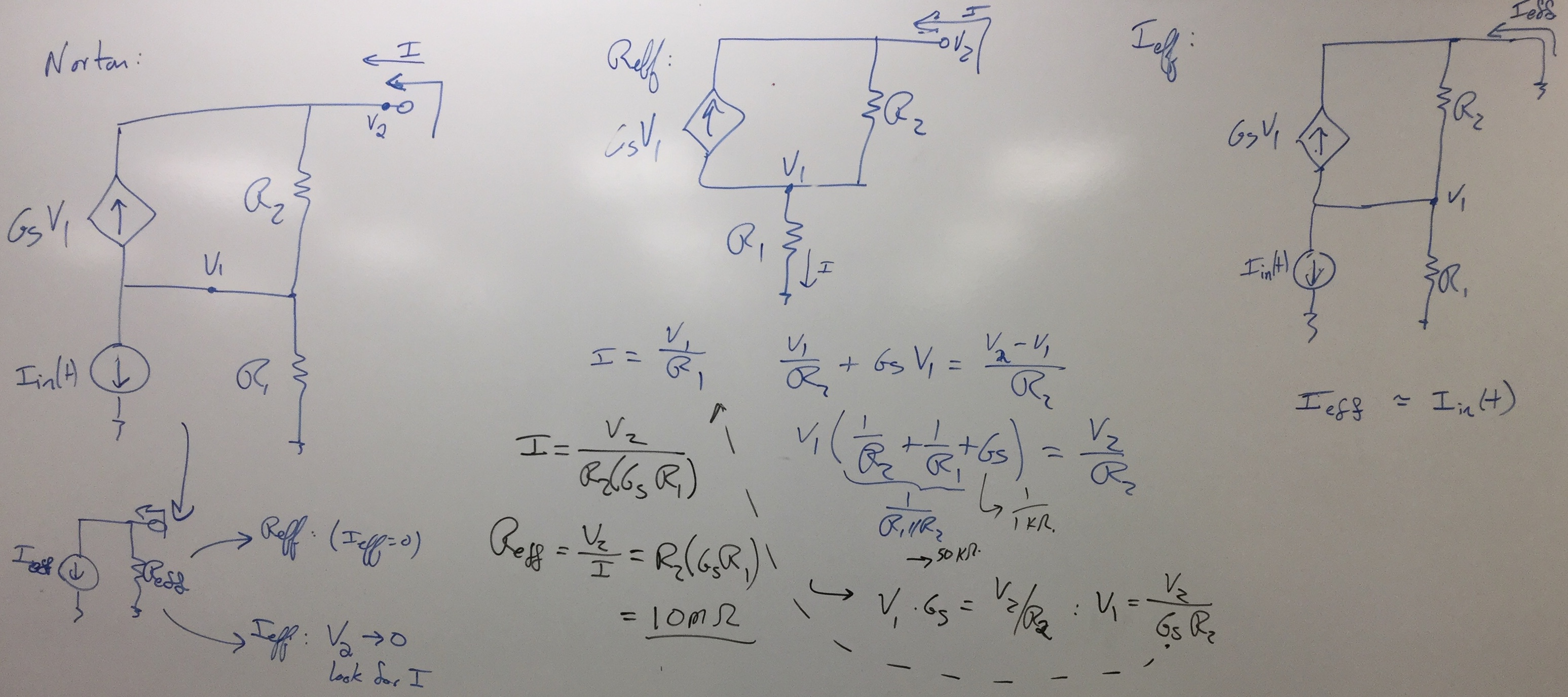
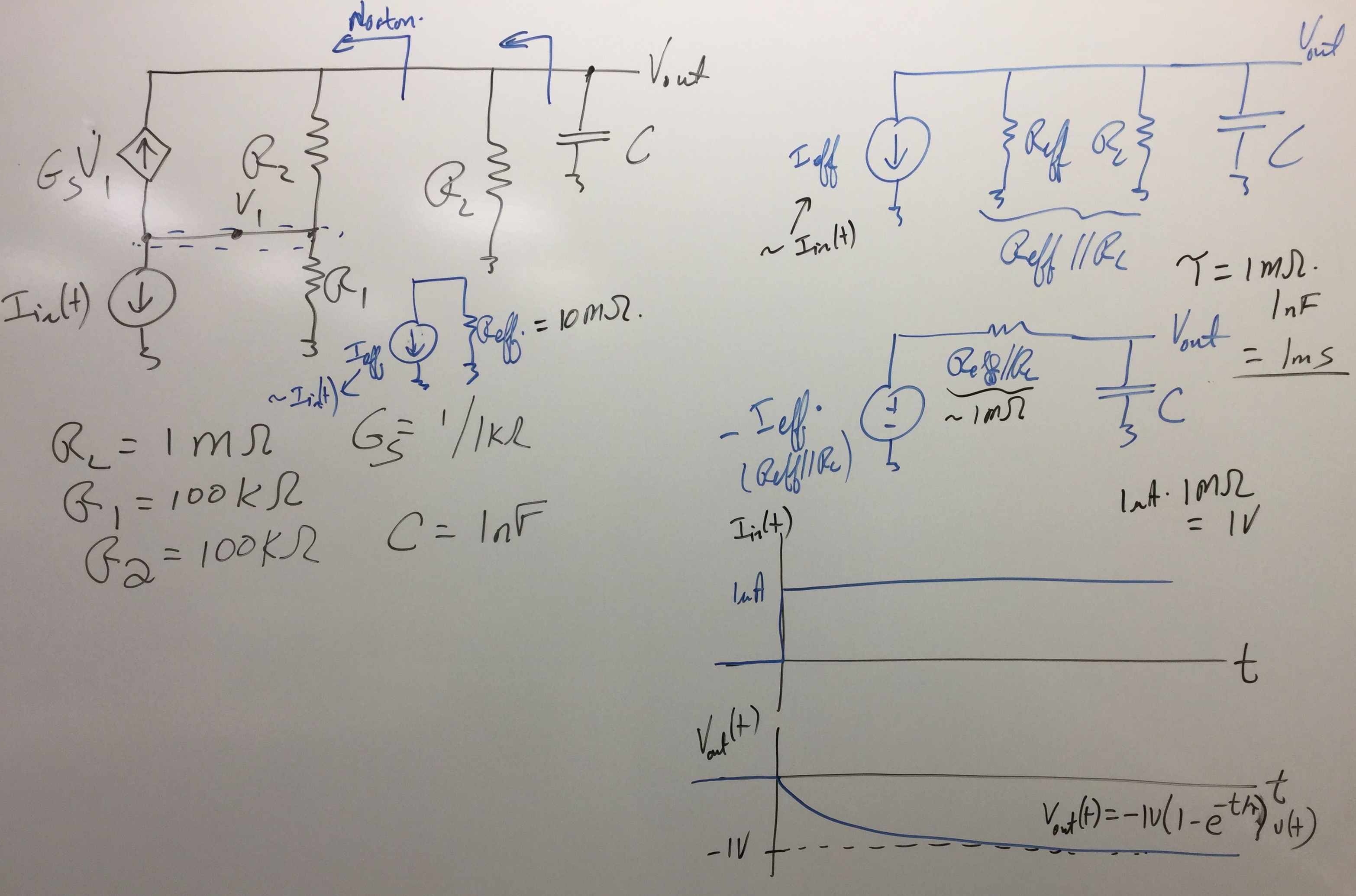
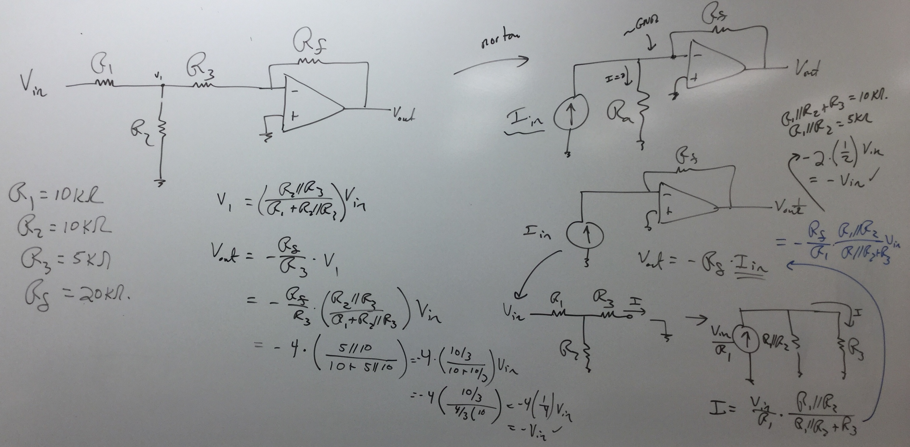
Thevenin-Norton OpAmp,
Capacitor-Focused Op-amp Circuit,
|
1,
2,
3,
4,
5,
6,
7,
8,
9
| |
Oct 1:
|
1 & 2 Order Circuit
|
Example
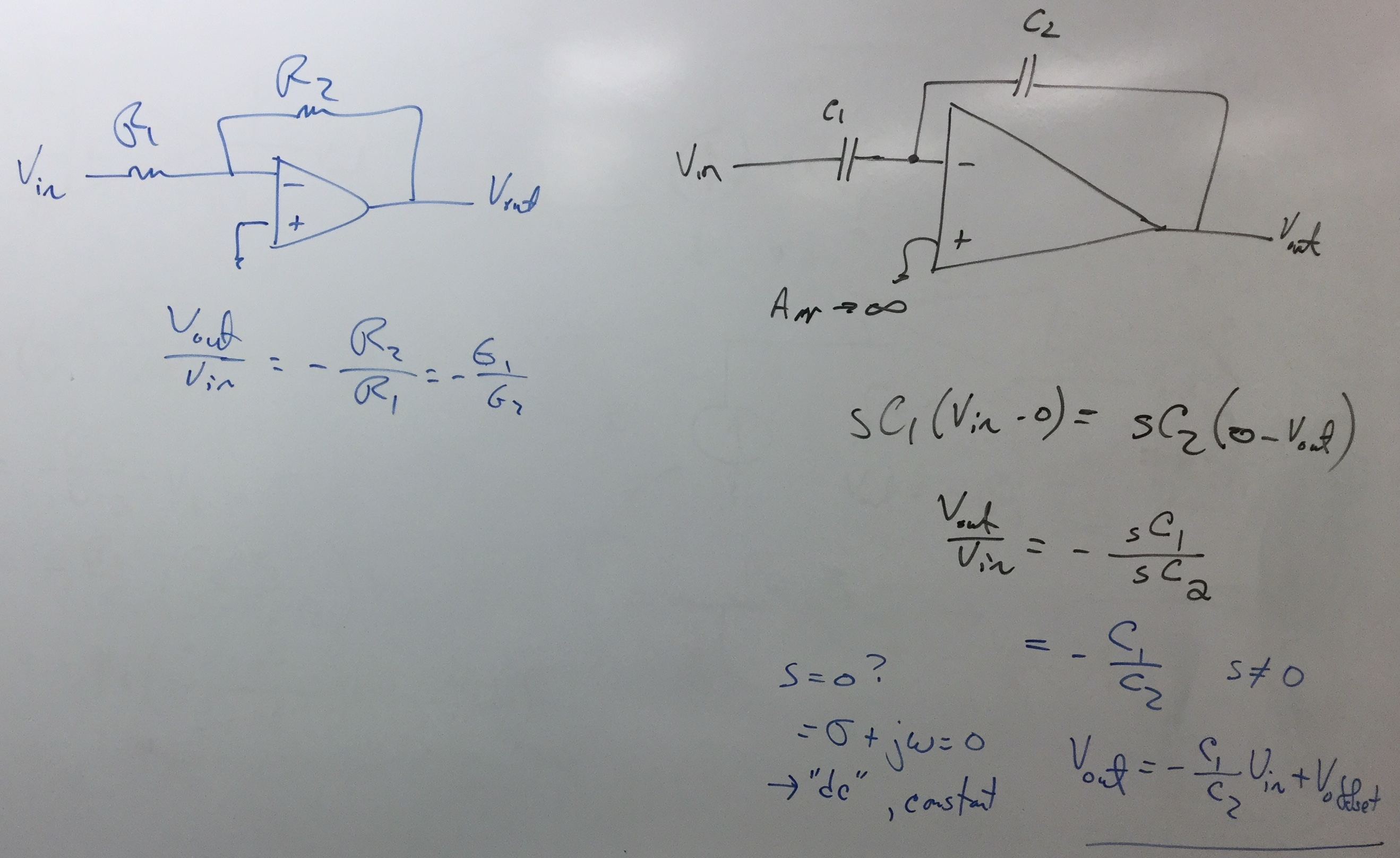
1st Order Op-Amp Step Response
2nd Order RC Circuit
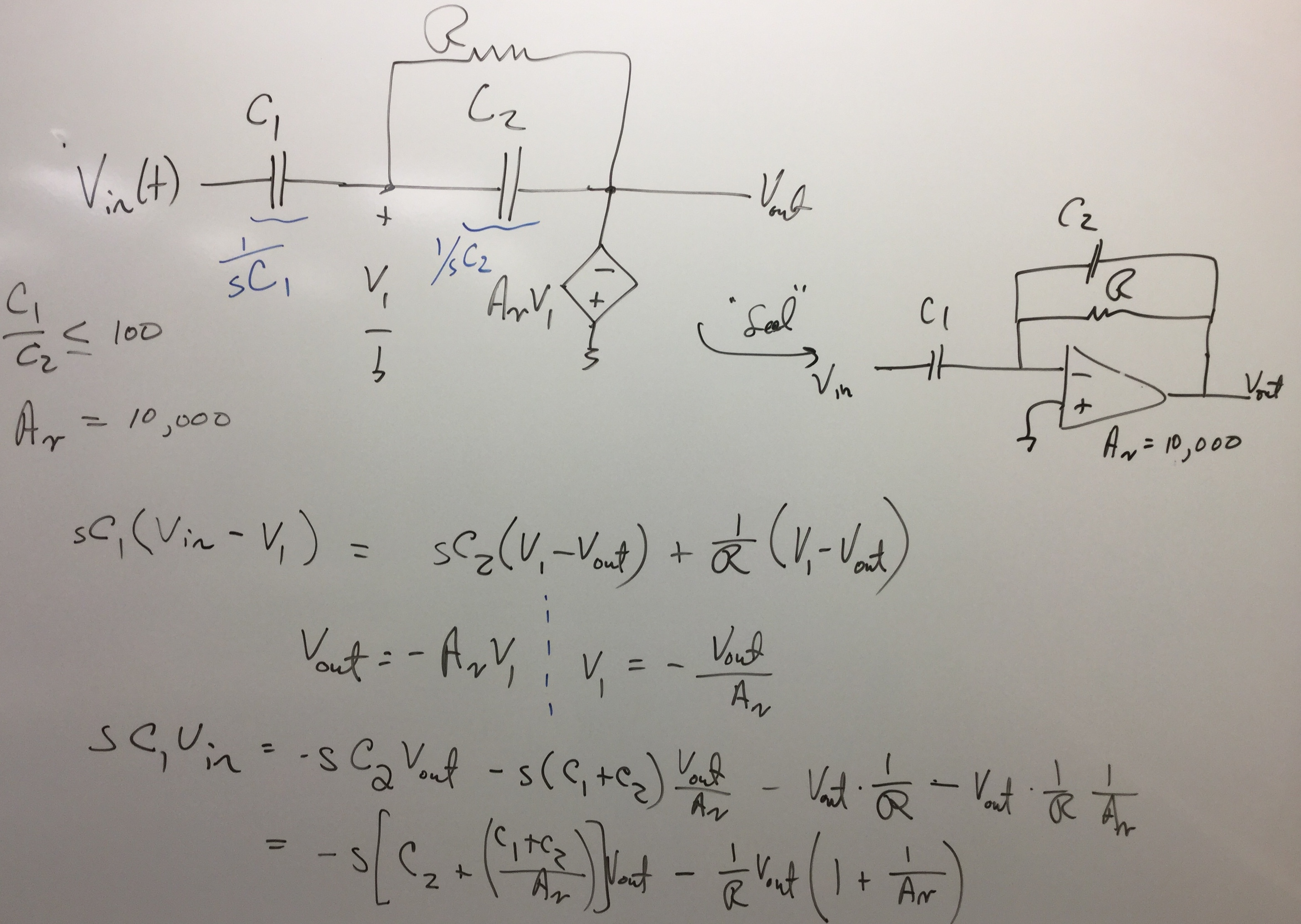
C-R Op-Amp Example
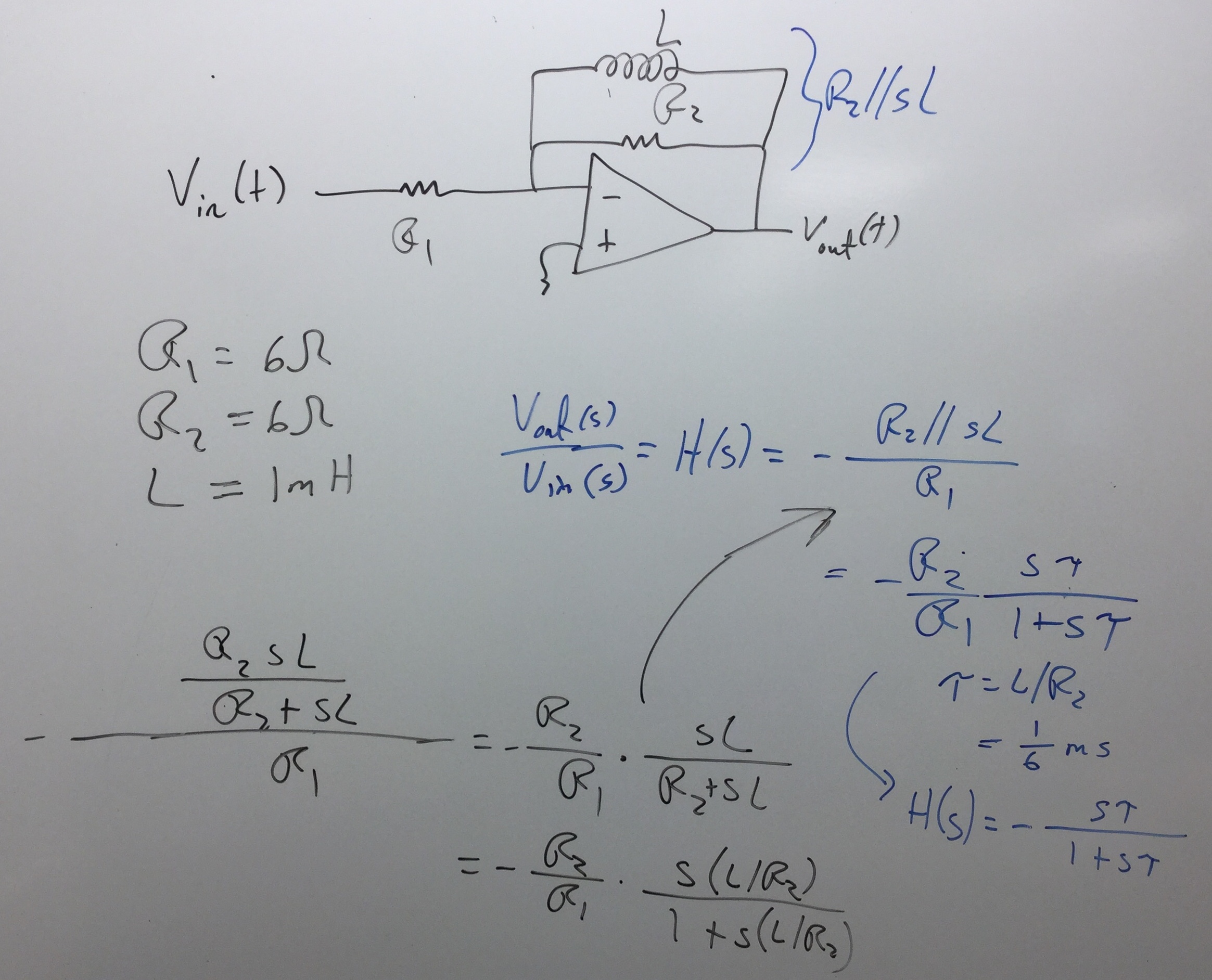
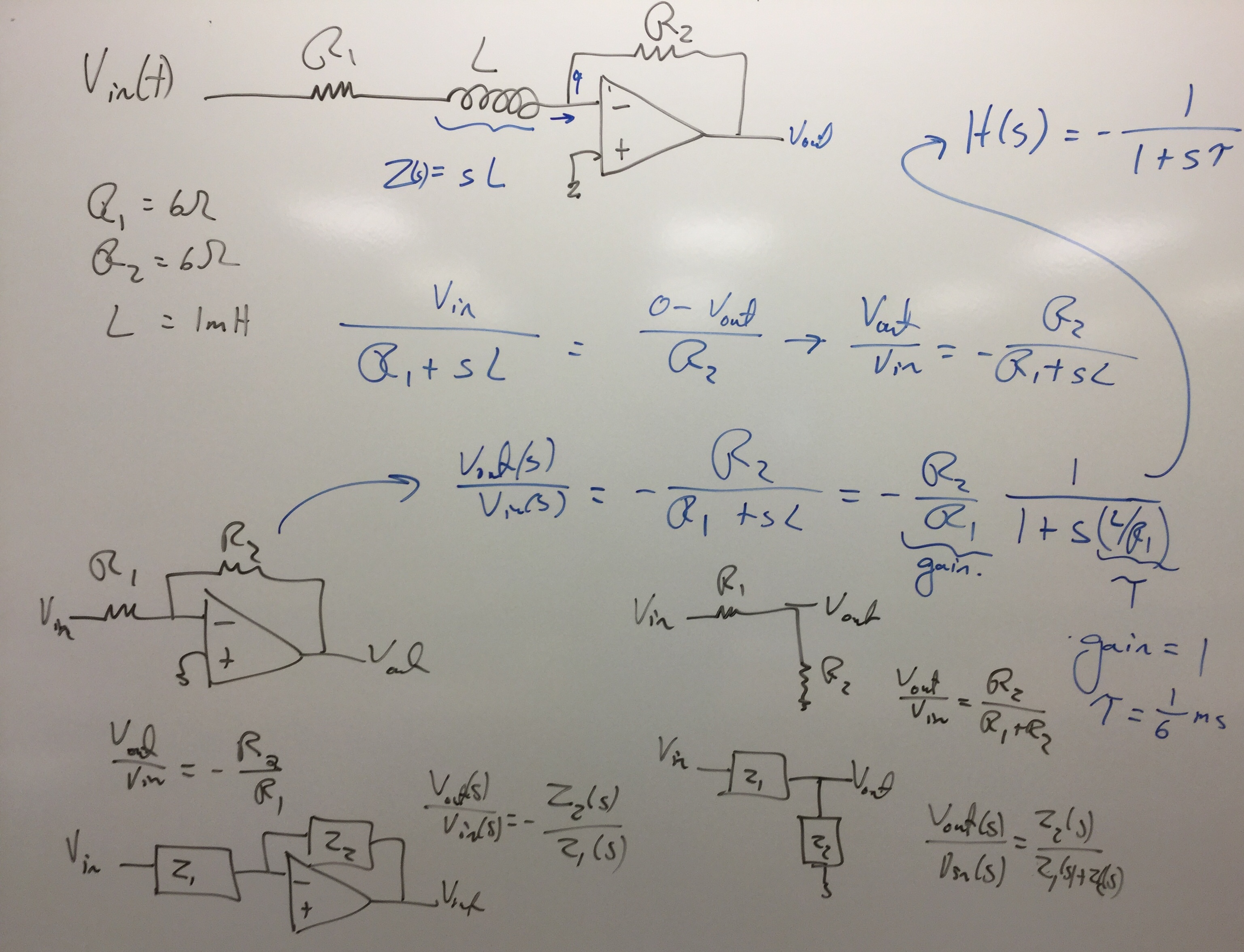
Op-Amp Inductor 1st
Thevenin Equivalent for Inductor-R circuits
|
1,
2,
3,
4,
5,
6,
7,
8,
9,
10,
11,
| |
Oct 6:
|
Unit Review
|
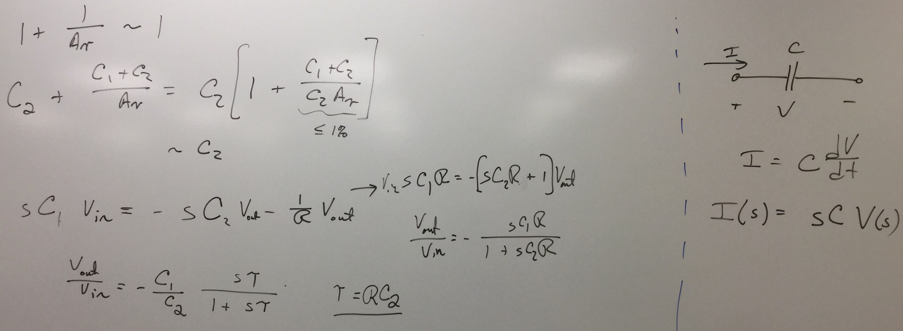
Middlebrook R-C Circuit
Capacitive Amp Circuit
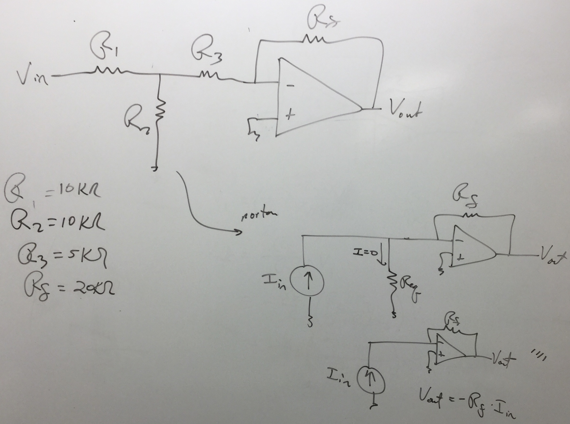
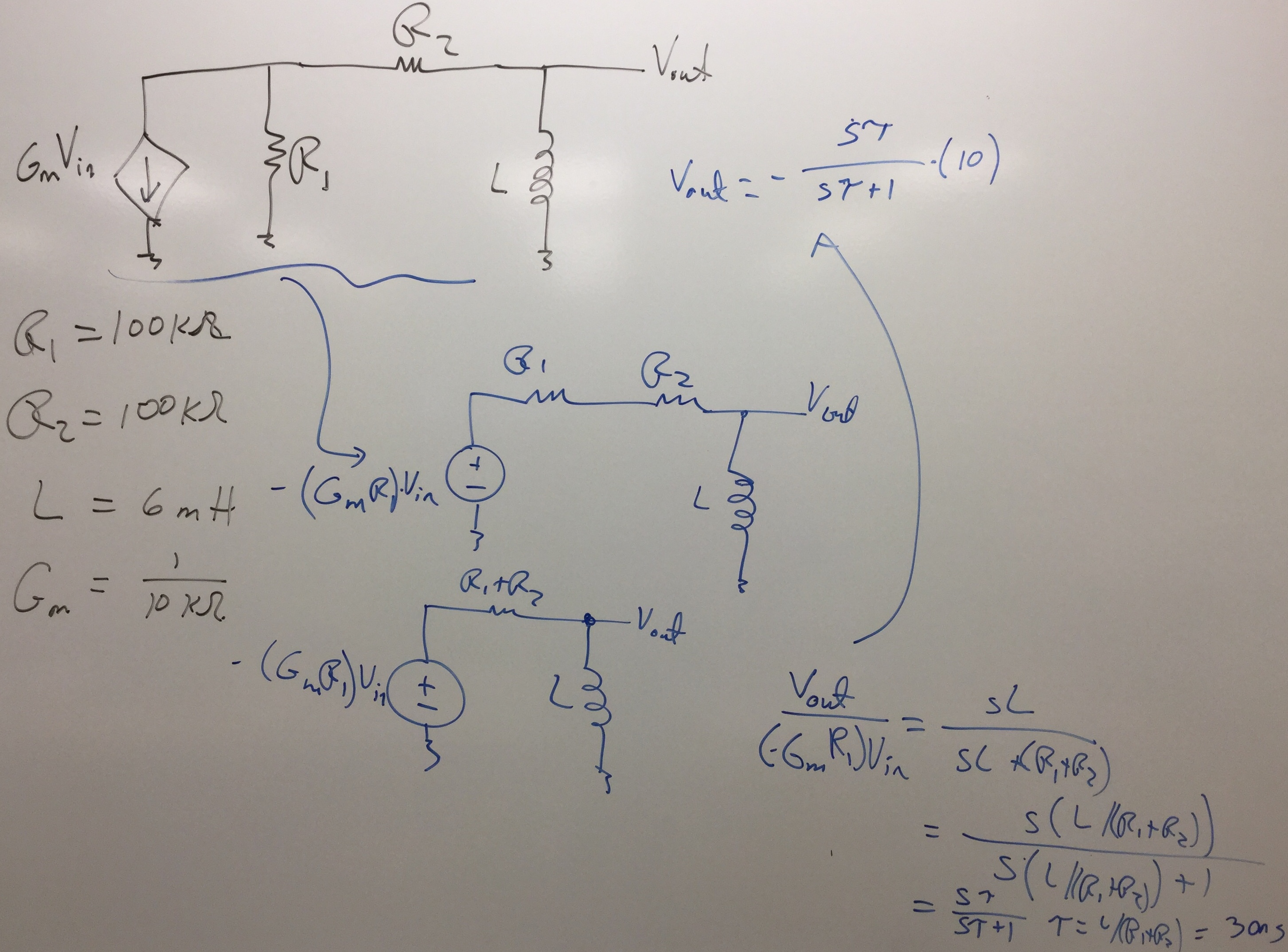
L-R Norton Op-Amp circuit
|
1,
2,
3,
4,
|
Unit 2 finishes with the
exam on Oct 8 (Thursday).
Most of the slides in
.pdf version from the taped lectures above
Reading
A few class items will be useful for this unit:
- Tables on Laplace Transforms:
Table 1,
Table 2
and
Table 3.
- Fourier Transform
Table.
- Exam 2, Spring 2019 with tentitive answers
pdf.
There can always be an answer that is not correct, so double check.
-
Exam 2, Spring 2020 with highlighted answers
pdf.
There can always be an answer that is not correct, so double check.
- Wikipedia's
page
on instrumentation amplifier using three op-amps.
- Random Slides on Laplace from other places:
1,
2,
3,
4.
- Some useful material from Linear Circuits course at Arizona State University
(EEE 202)),
Including good review on circuit analysis techniques
(pdf)
Basic linear ODEs
(pdf),
and Laplace Transforms
(pdf).
Additional Taped Lectures by Others :
For the second unit, there are a few parts of the textbook
that might be helpful to read for the discussions:
- Time dependant circuits with one state variable.
These circuits are mostly resistive networks with a single capacitor
or a single inductor.
Often these circuits require doing one or multiple resistive circuit
solutions to easily solve the time-dependant behavior
when switching a single voltage into the circuit (e.g. step response).
These circuits are developed in Chapter 8, as well as Chapter 7.9.
- Introduction to Op-Amp Circuits: Chapter 6.
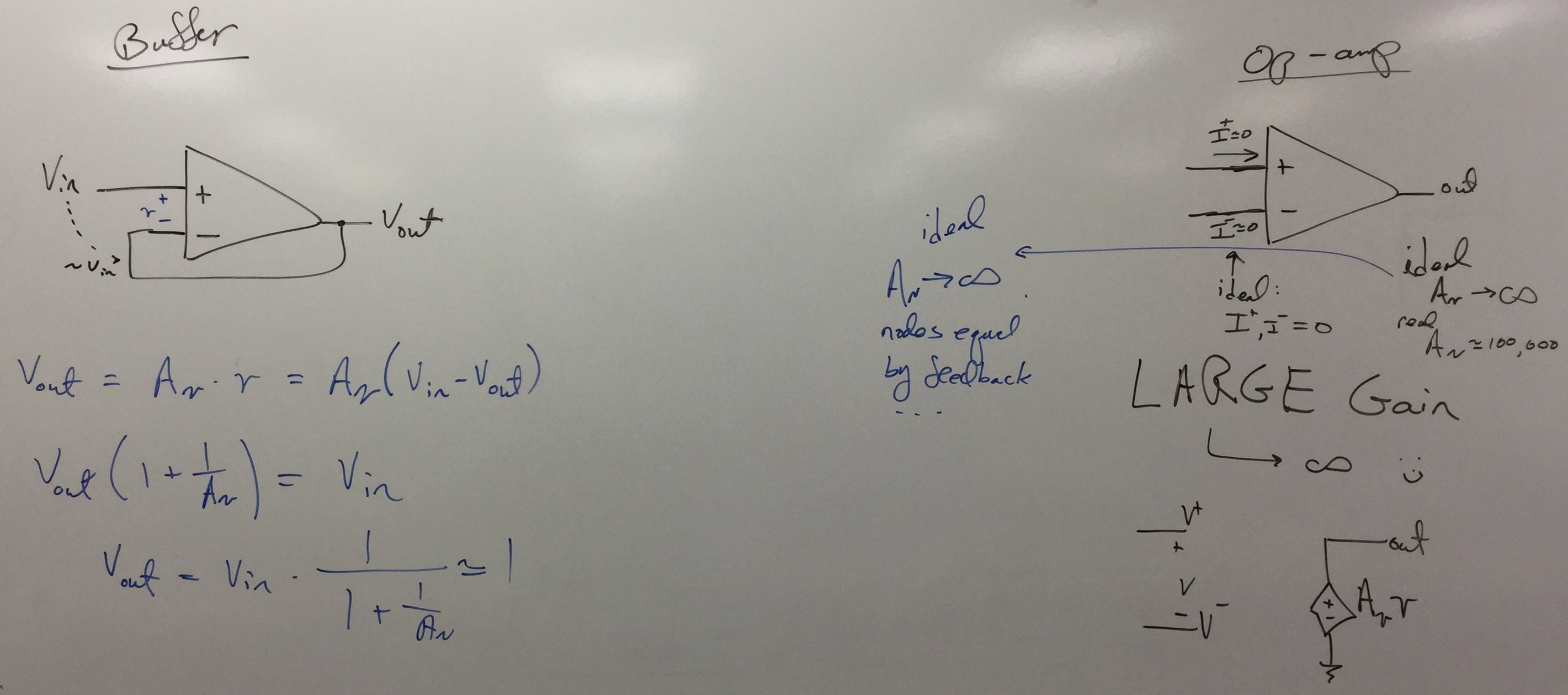
This unit we start our discussions of ideal op-amps,
devices when ideal, are a voltage-controlled voltage source
with huge gain between the input voltage and the output voltage.
The net effect is that the two terminals are nearly equal even though they
are not connected.
-
The response of a first-order circuit to a arbitrary input requires solving
the resulting differential equation for that signal.
Further, in practice, we have circuits that have more than
one capacitor and/or more than one inductor.
We need a generalized method for solving linear circuits,
a method developed by Heavyside around the turn of the 20th century,
who effectively created a general method for solving linear differential equations.
The method is called the Laplace Transform.
These methods turn linear differential equations into algebraic equations
in a different mathematical space that can be transformed back into normal space.
Chapter 14 covers Laplace transforms, and we will focus on these techniques in this unit.
We will return to the other chapters, Chp. 9 - 13 in the third unit.
We will create transformed circuit models for linear elements,
transforming most circuit problems into a modified resistive elements.
Sections 14.2 - 14.5 goes through the mathematics for the Laplace Transform.
Understand this is math heavy and I would suggest skimming alot of the chapter,
look at 14.6, 14.7, and then read these sections again.
Section 14.6 discusses using Laplace techniques to solve the differential equations
that come from a linear circuit analysis.
Section 14.7 discusses directly analyzing linear circuits directly by Laplaced Transformed Elements.
In particular, you should look at pg. 693.
Section 14.8 generalizes these concepts to transfer functions.
Assigned Homework Problems
Problems to be Submitted
- Set 3, Due Sept 24:
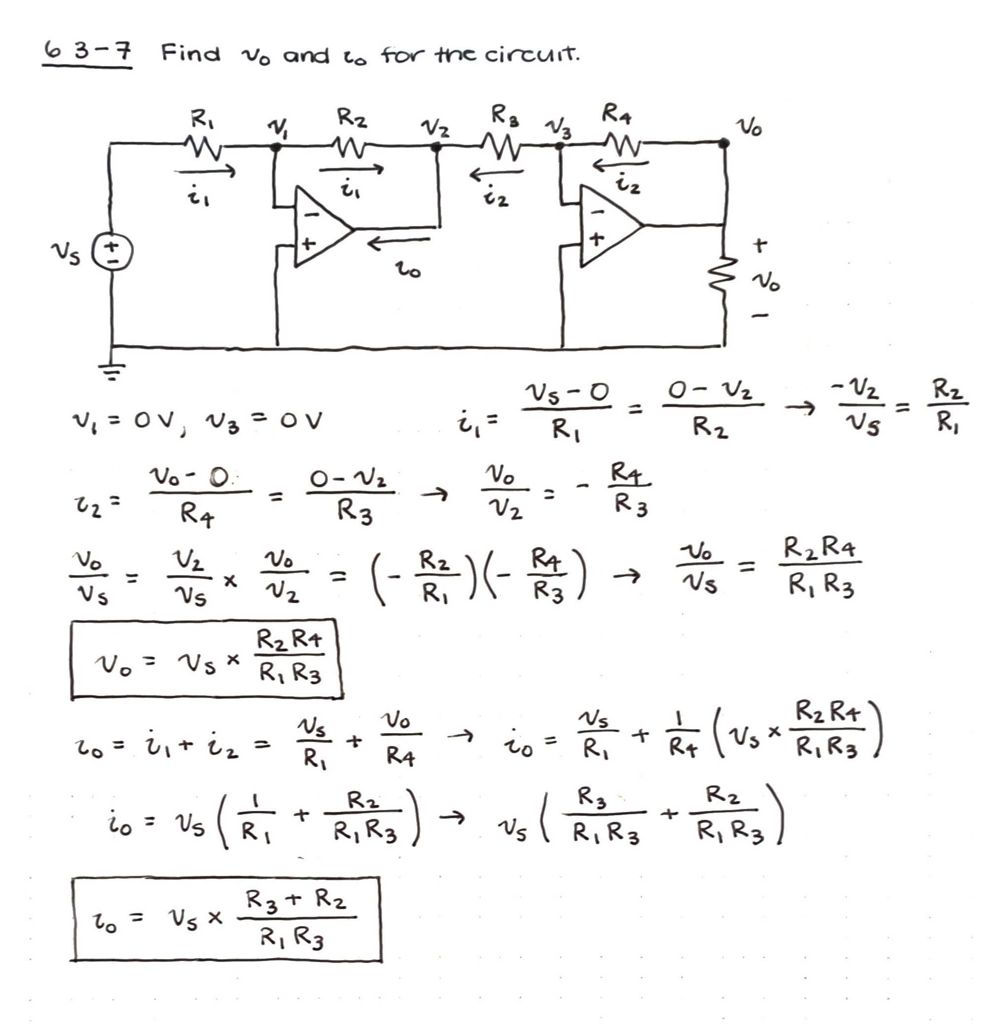
6.3-7
Solution,
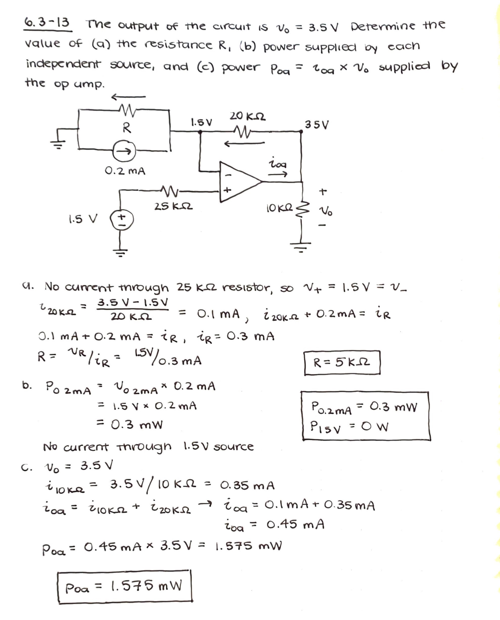
6.3-13
Solution,
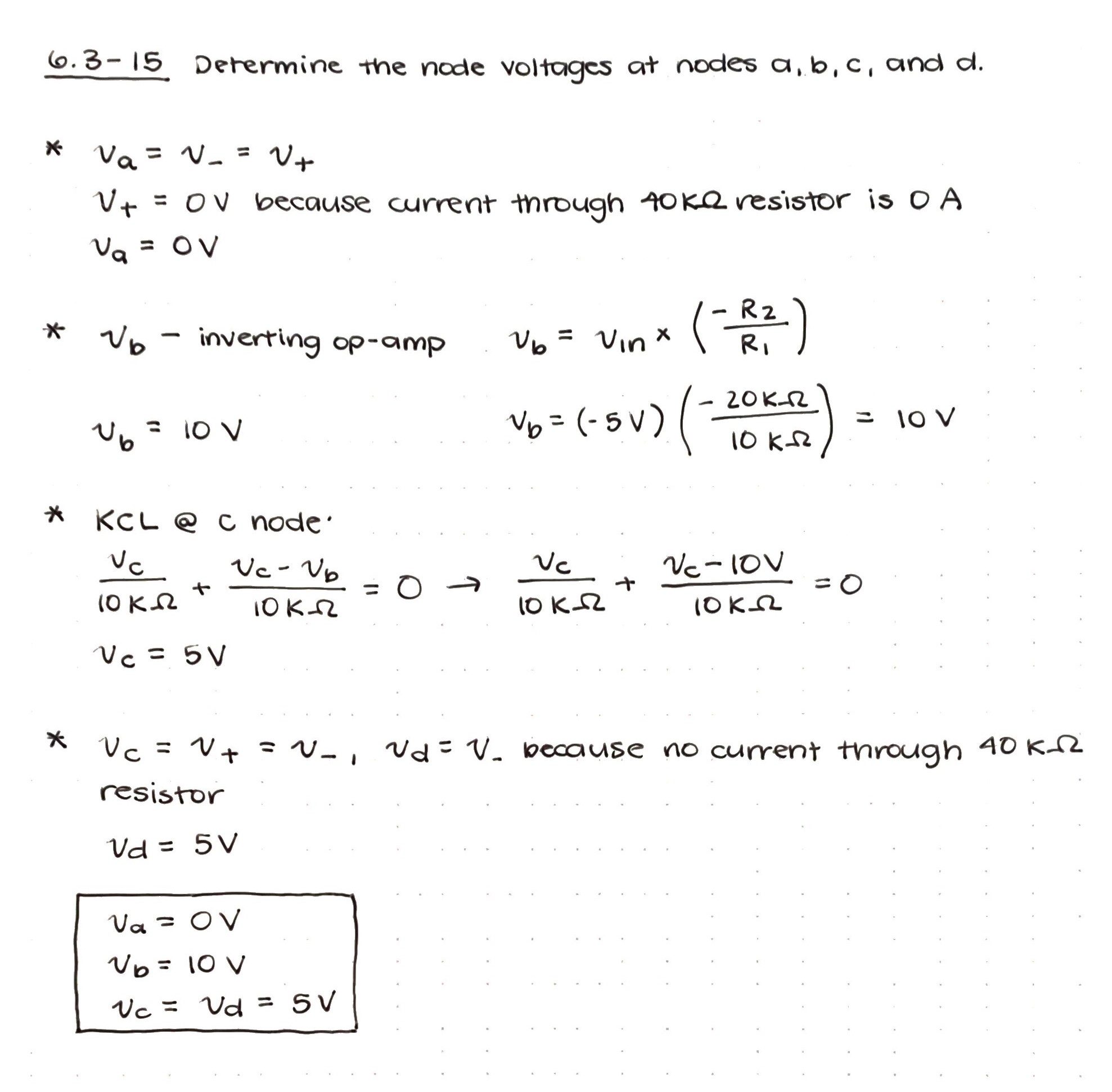
6.3-15
Solution,
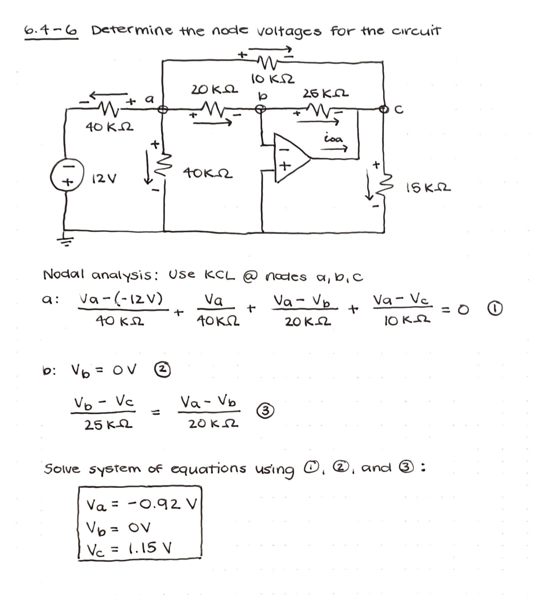
6.4-6
Solution,
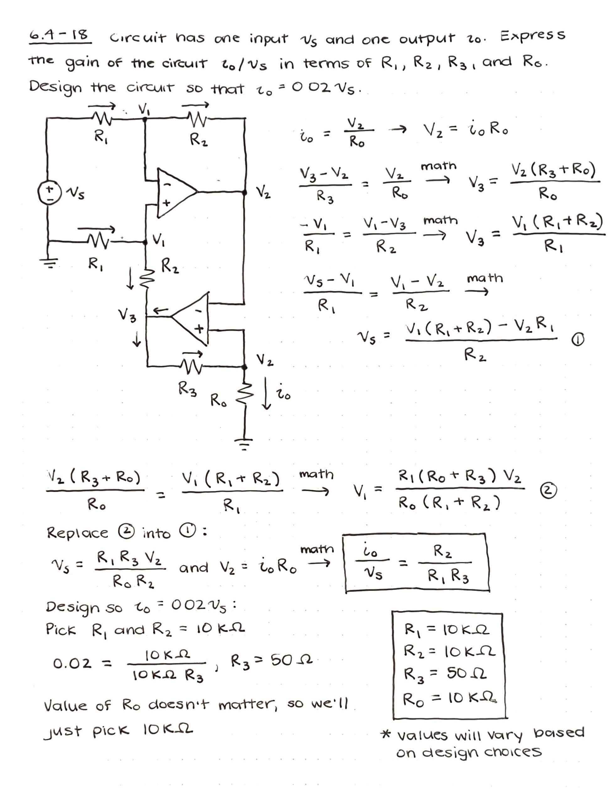
6.4-18
Solution,
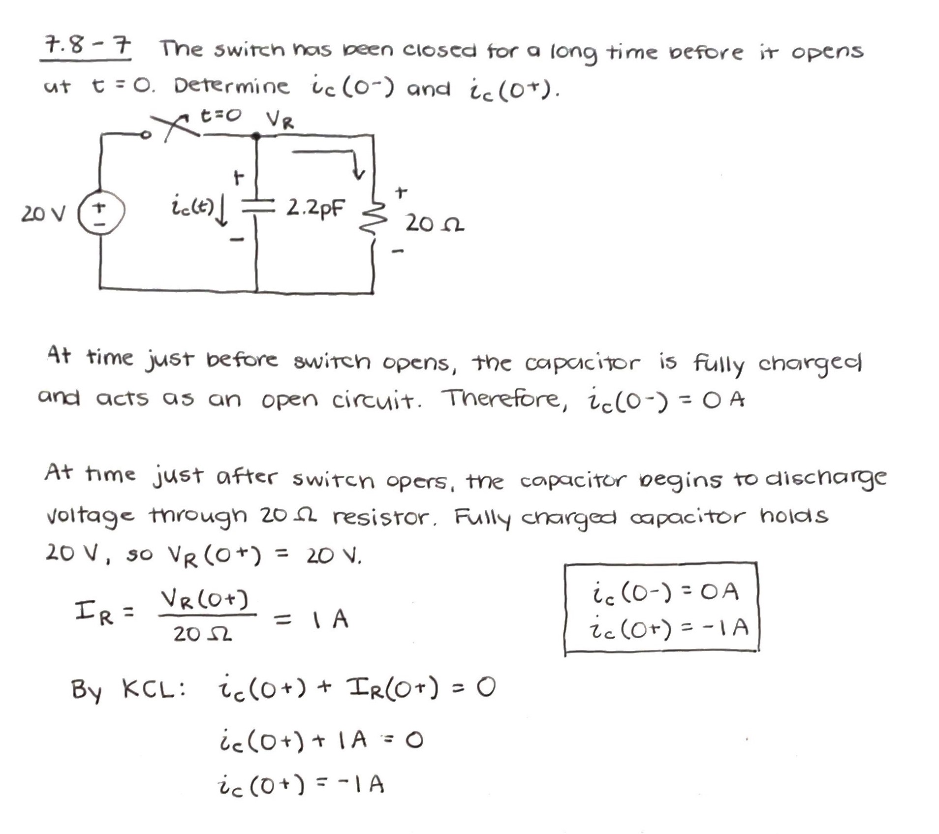
7.8-7
Solution,
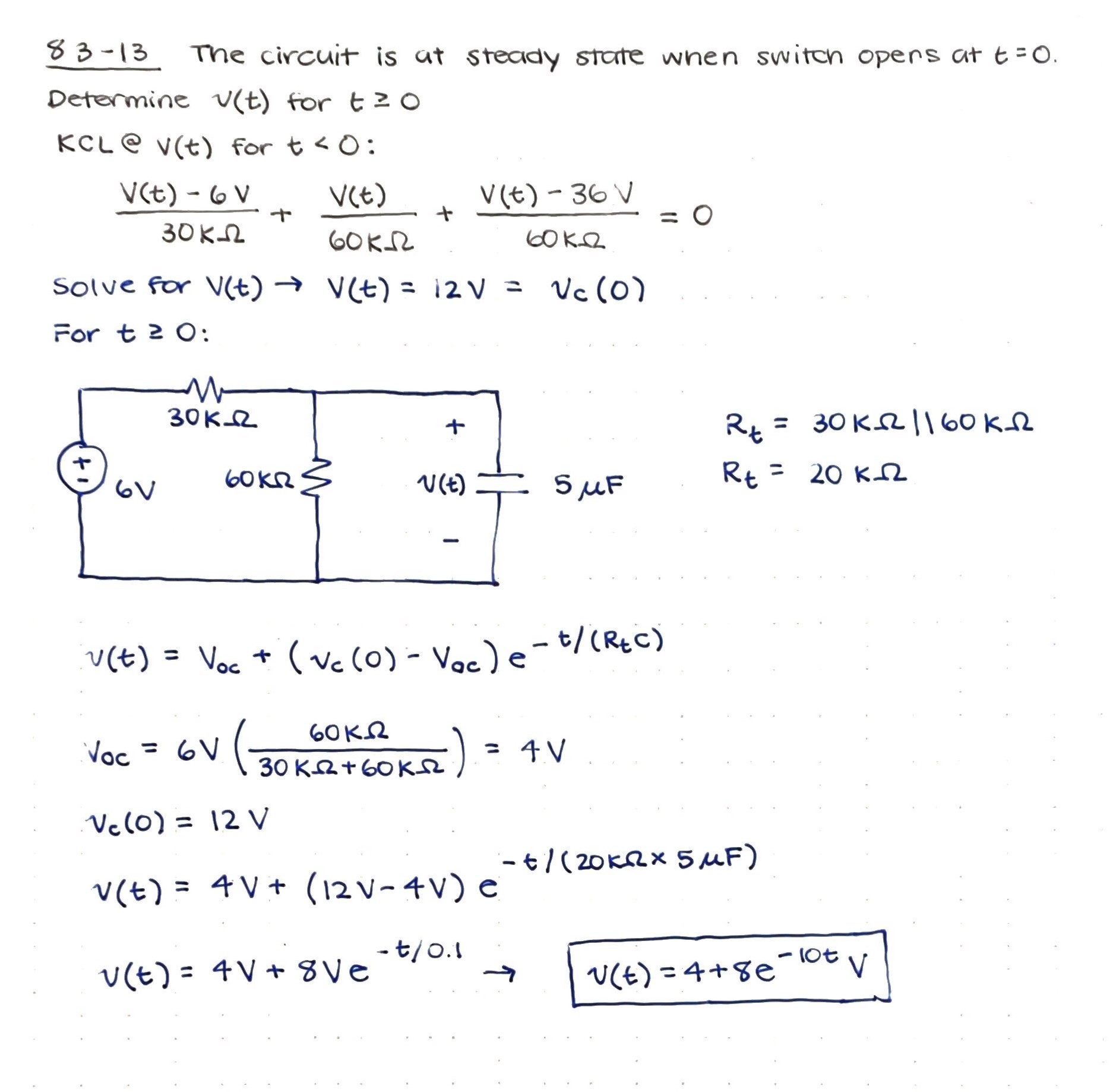
8.3-13
Solution
- Set 4, Due Sept 29:
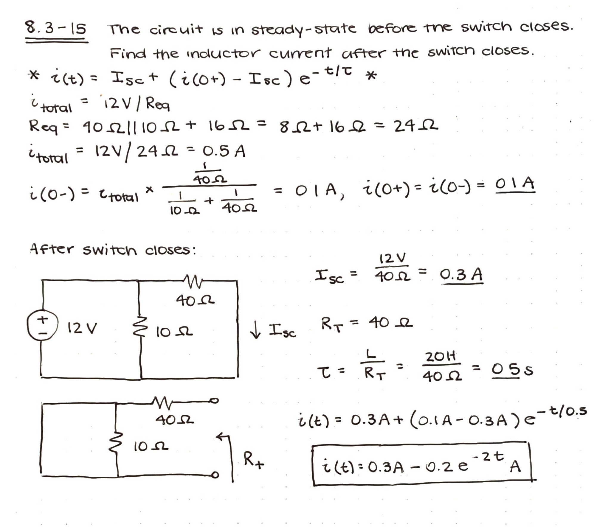
8.3-15
Solution,
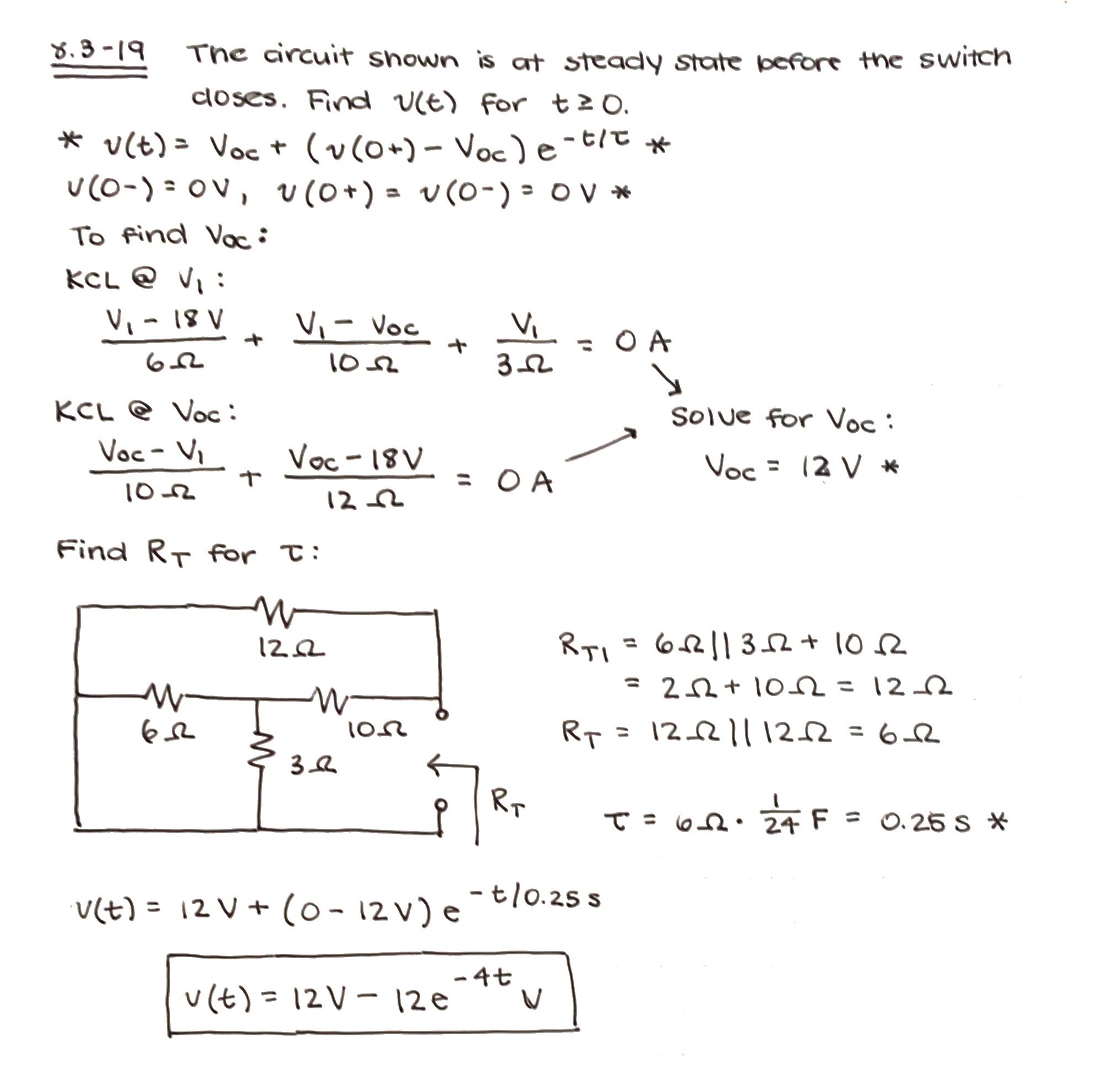
8.3-19
Solution,
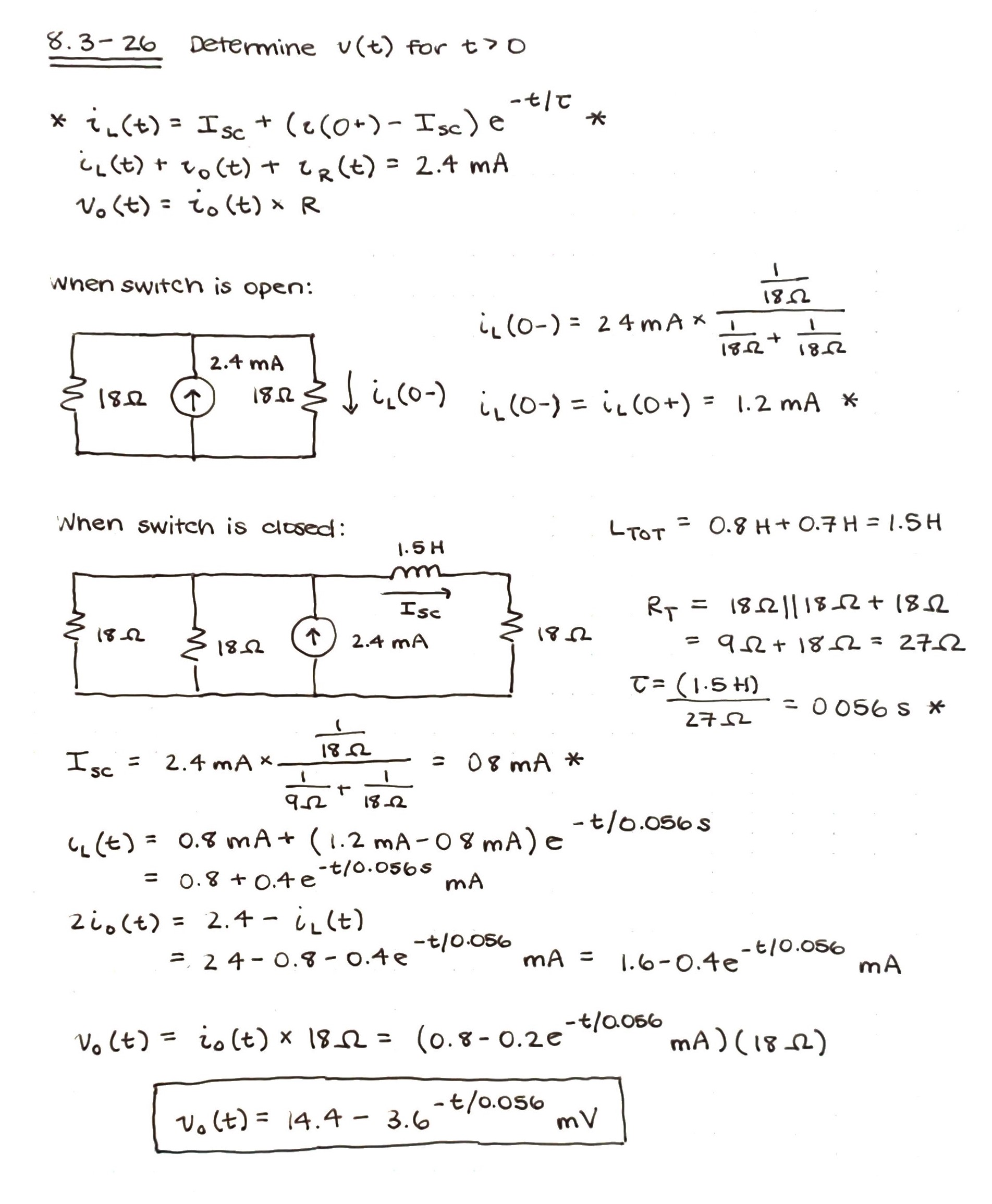
8.3-26
Solution,
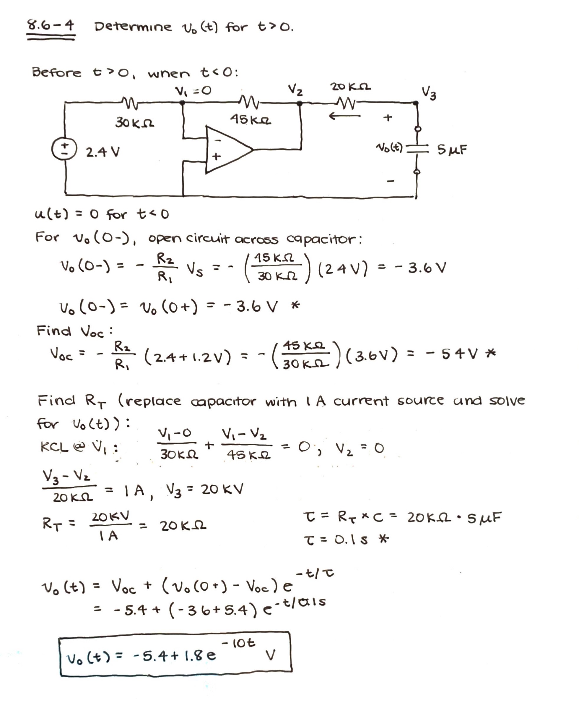
8.6-4
Solution,
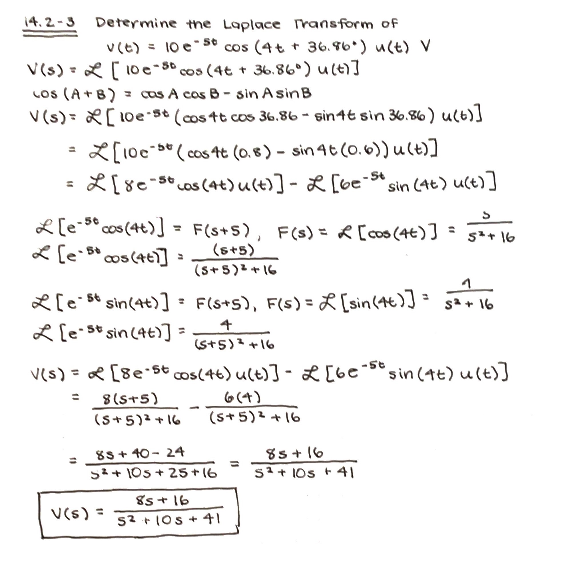
14.2-3
Solution,
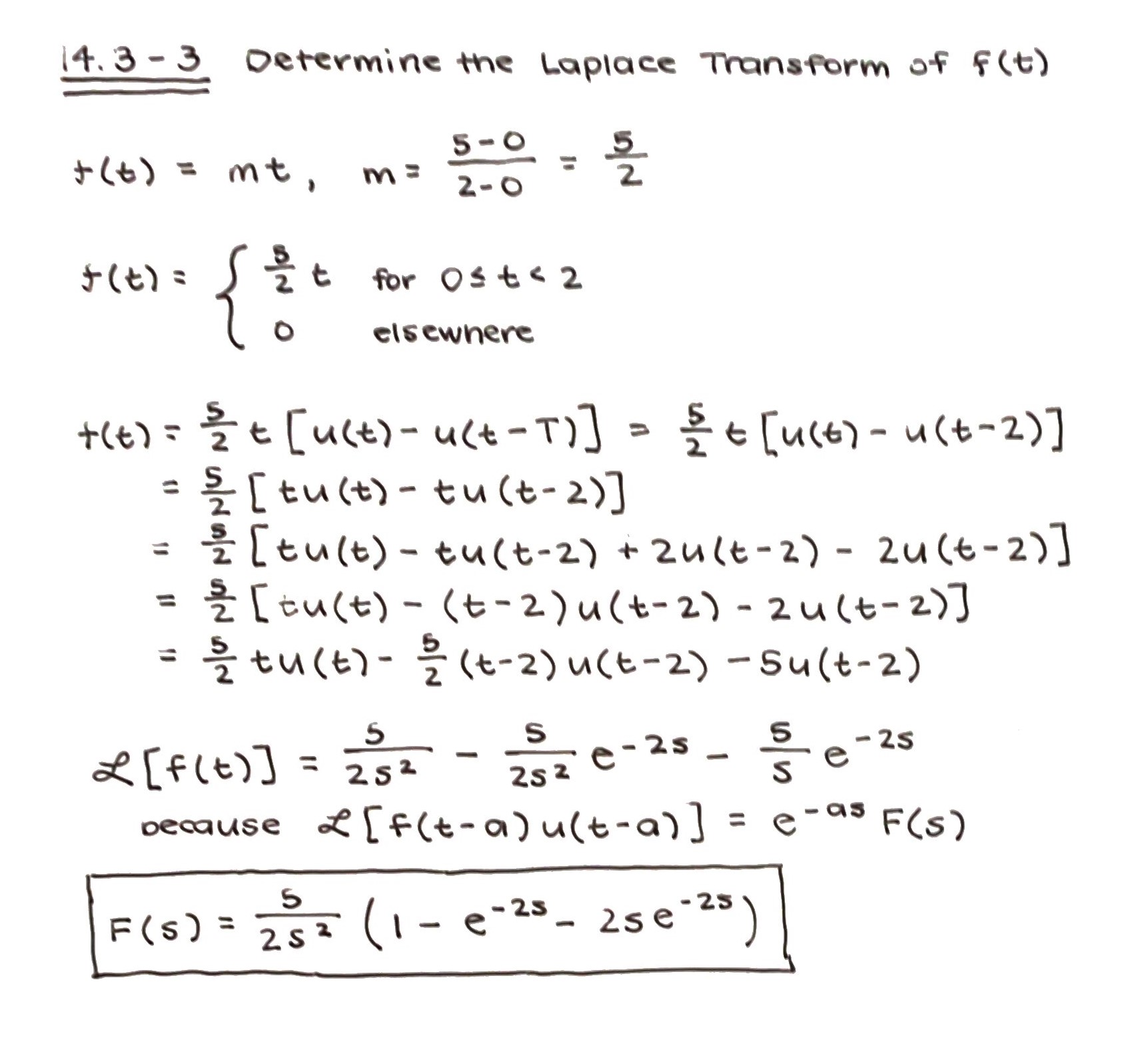
14.3-3
Solution,
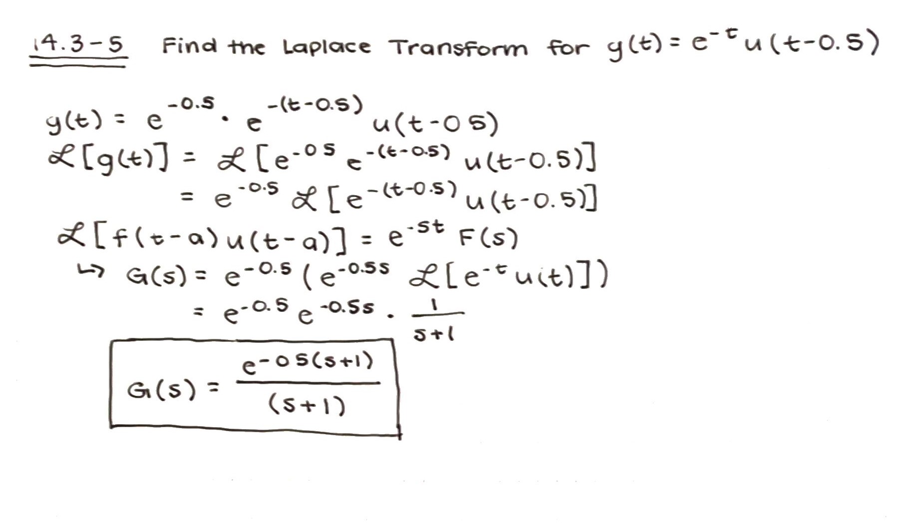
14.3-5
Solution,
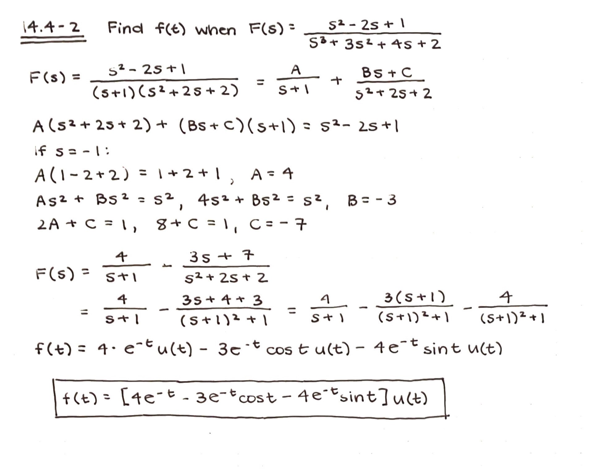
14.4-2
Solution,
- Set 5, Due Oct 6:
8.6-11
Solution,
8.6-25,
Solution,
14.4-5,
Solution,
14.5-2,
Solution,
14.7-3,
Solution,
14.7-7,
Solution,
14.7-13,
Solution,
14.7-17
Solution
Previous Problems and Solutions
You are expected to work through these problems during this unit.
The solutions are provided.
You should attempt these problems before attempting the submitted homework problems.
You should not submit any of these solutions.
Practice solving linear circuit problems tends to be very important to learning this material well.
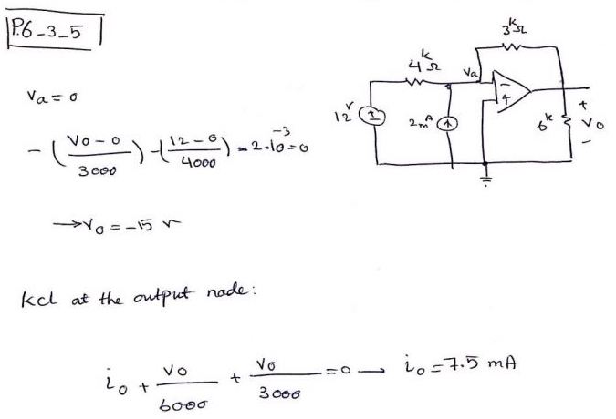
- P6.3-5
Solution ,
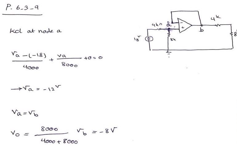
- P6.3-9
Solution ,
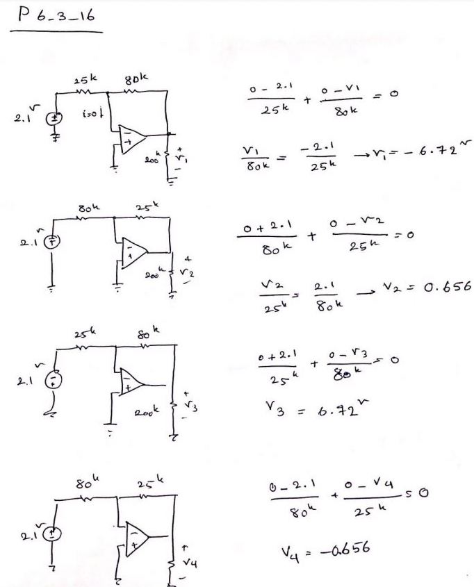
- P6.3-16
Solution ,
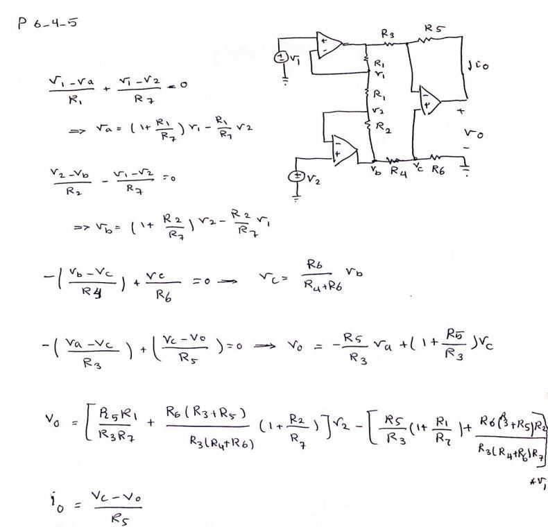
- P6.4-5
Solution ,
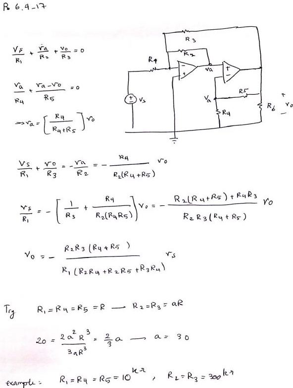
- P6.4-17
Solution ,
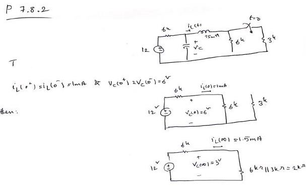
- P7.8-2
Solution ,
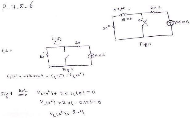
- P7.8-6
Solution ,
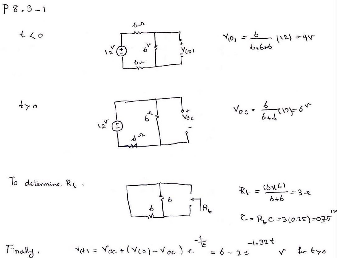
- P8.3-1
Solution ,
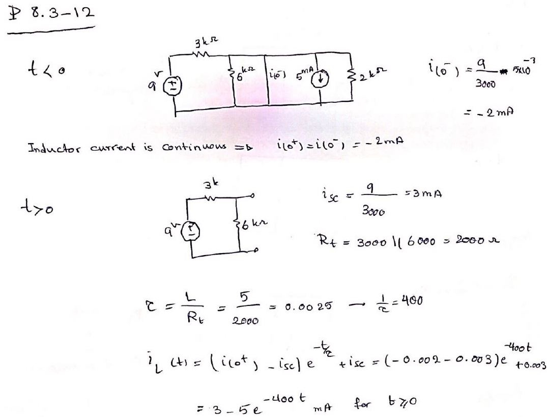
- P8.3-12
Solution ,
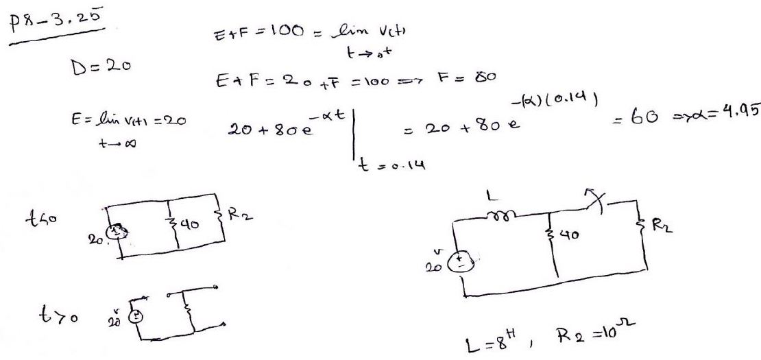
- P8.3-25
Solution ,
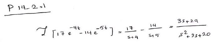
- P14.2-1
Solution ,
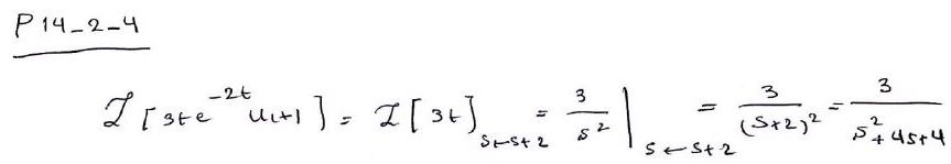
- P14.2-4
Solution ,
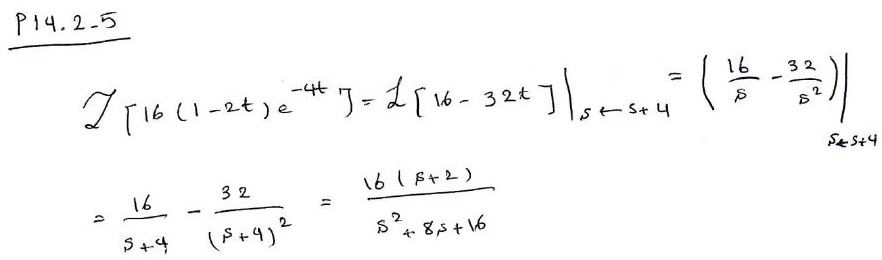
- P14.2-5
Solution ,
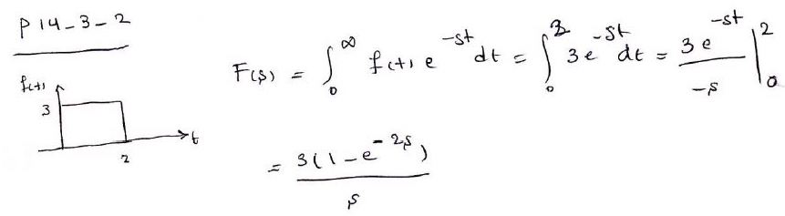
- P14.3-2
Solution ,
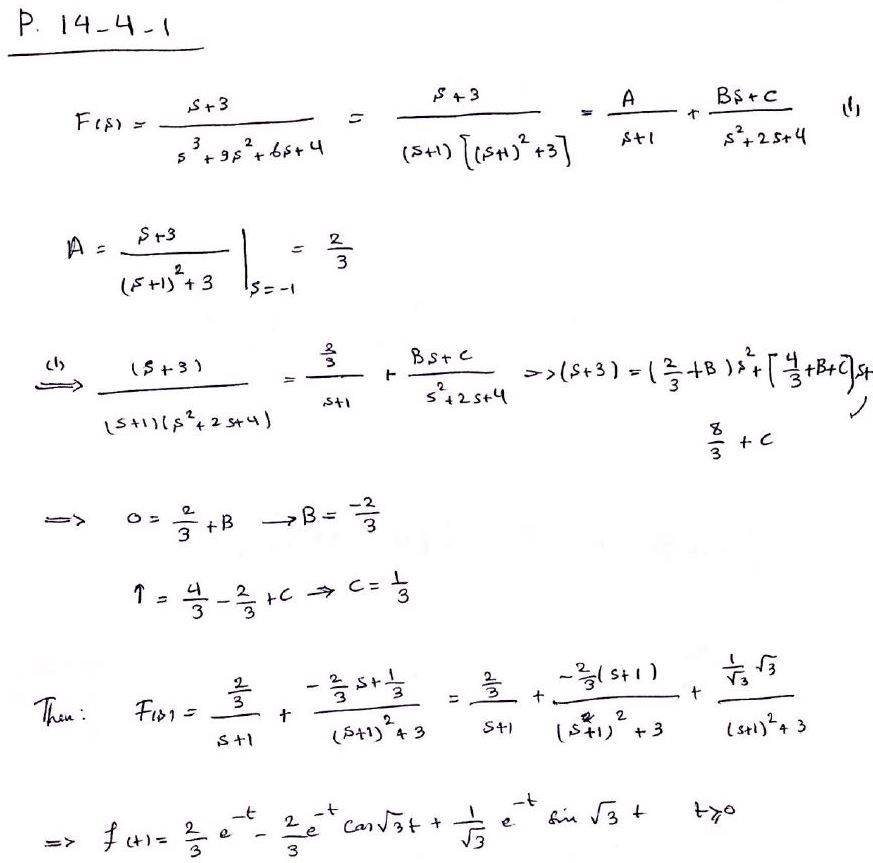
- P14.4-1
Solution ,
- P14.4-3
Solution ,
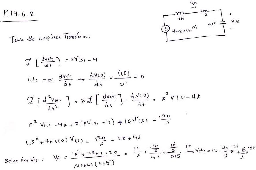
- P14.6-2
Solution
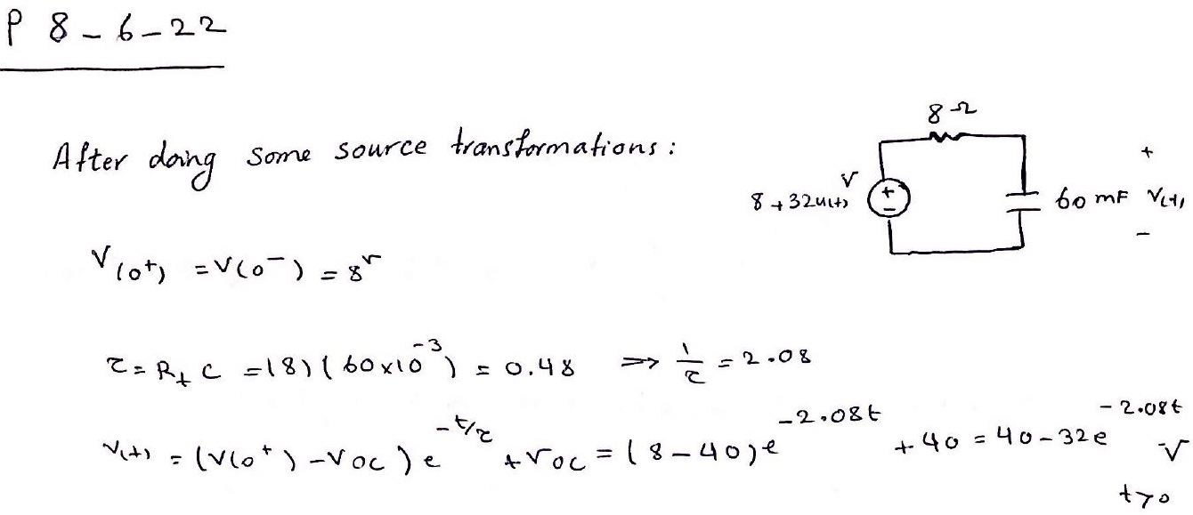
- P8.6-22
Solution ,
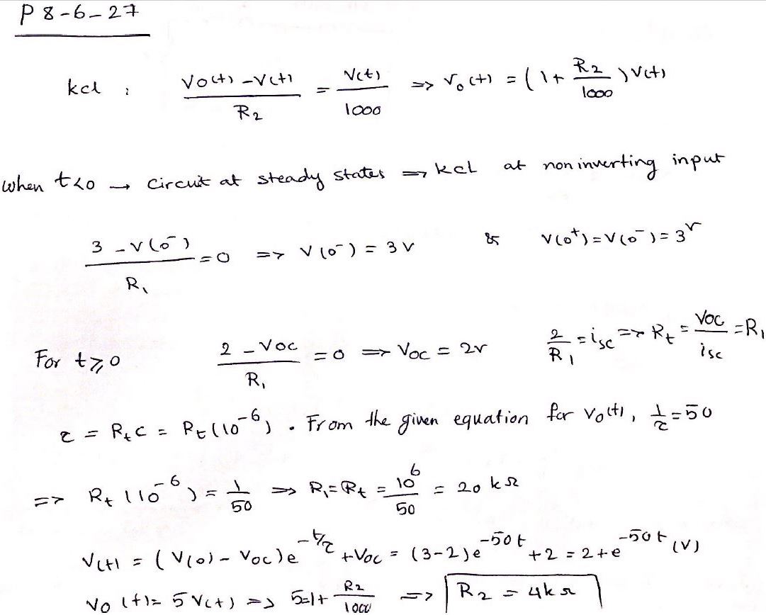
- P8.6-27
Solution ,
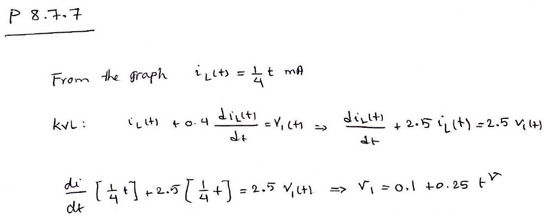
- P8.7-7
Solution ,
- P14.6-3
Solution ,
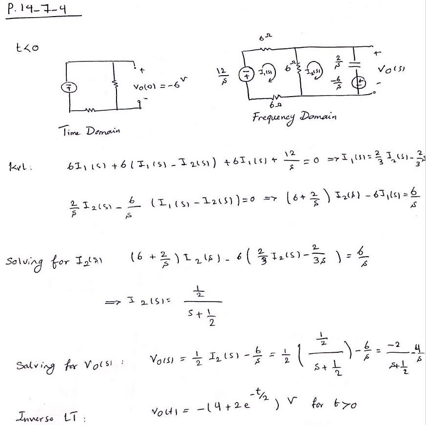
- P14.7-4
Solution ,
- P14.7-12
Solution Part 1 and
Solution Part 2 ,
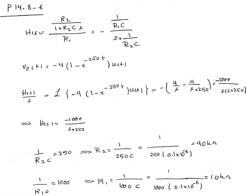
- P14.8-6
Solution
Project Items
This project primarily gets the students comfortable with measurement and resulting analysis of
time-domain (Resistor-Capacitor) circuits.
|
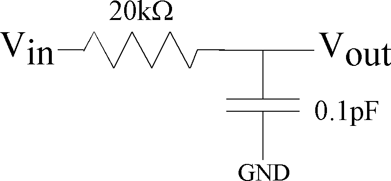
Figure 1: First-order Resistor--Capacitor Circuit for lab measurement.
The precise values of the Resistor and Capacitor are not essential,
e.g. 0.1pF may not be an ideal choice.
One should choose proper values to see the dynamics
using your particular data aquisition system.
|
Remember plots and data analysis are done in MATLAB / Scilab;
please don't include your code in your writeup.
You will submit one writeup per group electronically to the professor
(both individuals may submit the same report twice in Canvas if both names are on both documents).
Preferred naming of the submitted document: "Project2_LastName1_LastName2".
|
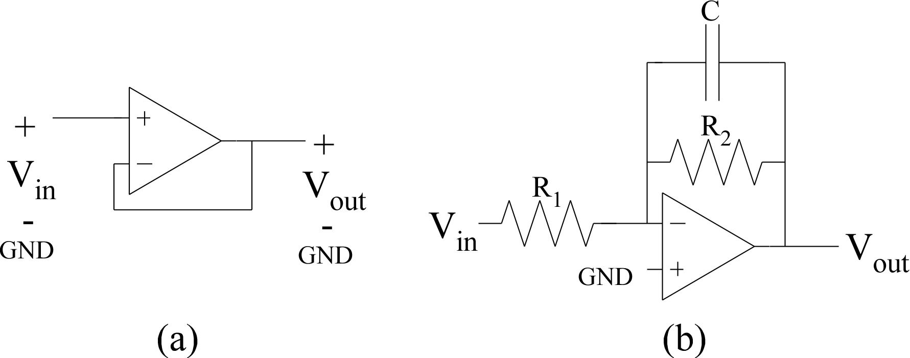
Figure 2: Op-Amp Circuits for lab measurement.
(a) An Op-Amp buffer circuit.
(b) A First-order Op-Amp Resistor--Capacitor Circuit.
|
- Set up the First-Order RC circuit that you find in Fig. 1.
You will want to use an Op-amp buffer (Fig. 2a) between the output and your instrumentation.
First check that the buffer is working, doing a simple sweep of Vin
versus Vout.
Then check that the full circuit is working by doing a simple sweep
of the resistor input voltage vs. Vout.
you will notice that the output voltage should approximately equal the input voltage.
The input voltage can be swept for this measurement between 0 and 3V or 5V.
You should have a gain = 1.
Curve fit this value, and discuss any differences.
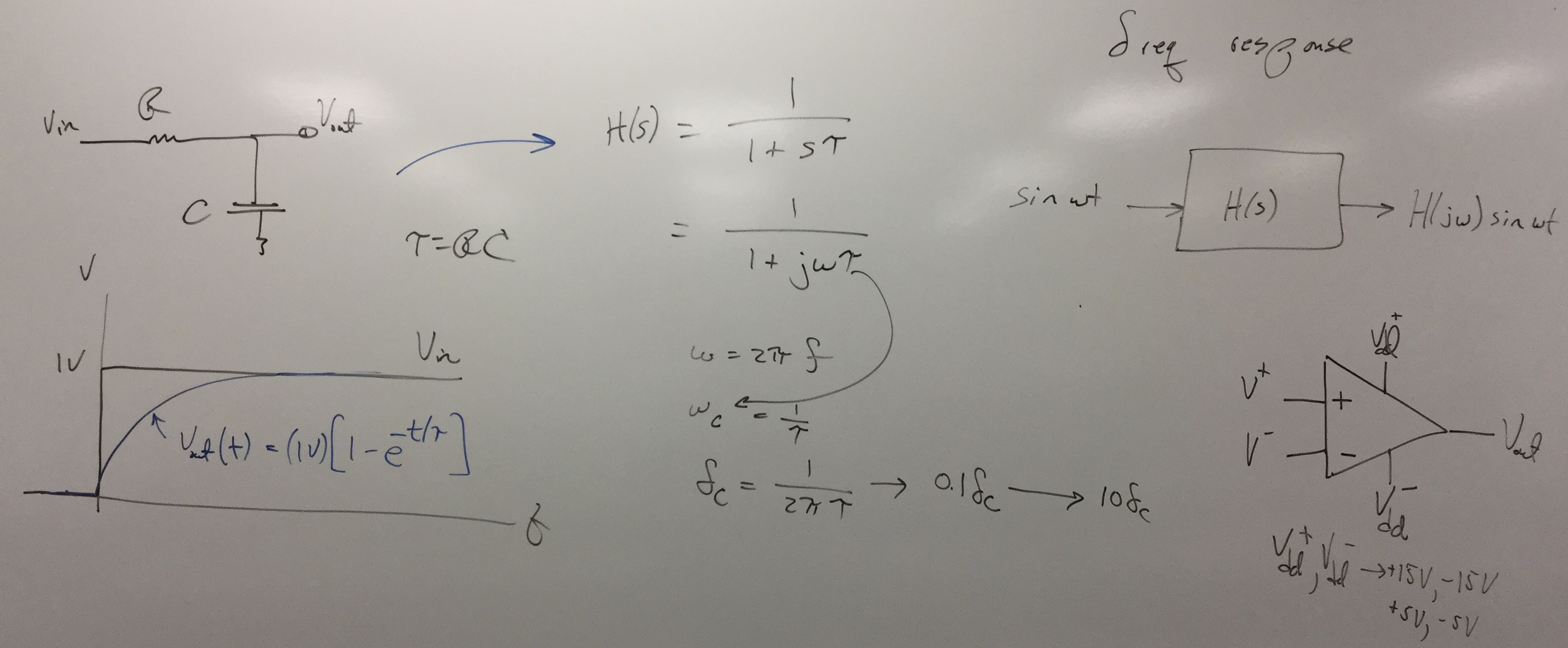
- Perform a step response (Fig. 1):
This means you have a square wave input and look at the resulting output voltage.
Put in an input step between 0.5V and 1.5V. You have a dc voltage of 1V.
Analytically solve for the RC timeconstant and for Vout response with time,
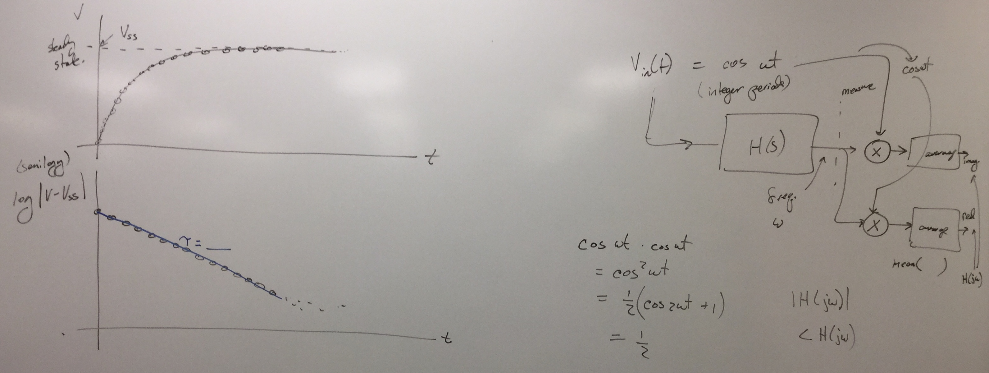
as well as use your experimental data to experimentally measure the RC timeconstant.
You will perform a curve fit for the resulting time constant ,
a curve fit to the exponentially decreasing and exponentially increasing data.
Do the two time-constant values agree?
You need to include a plot of the measured data with curve fits for the time-constant of the measured data.
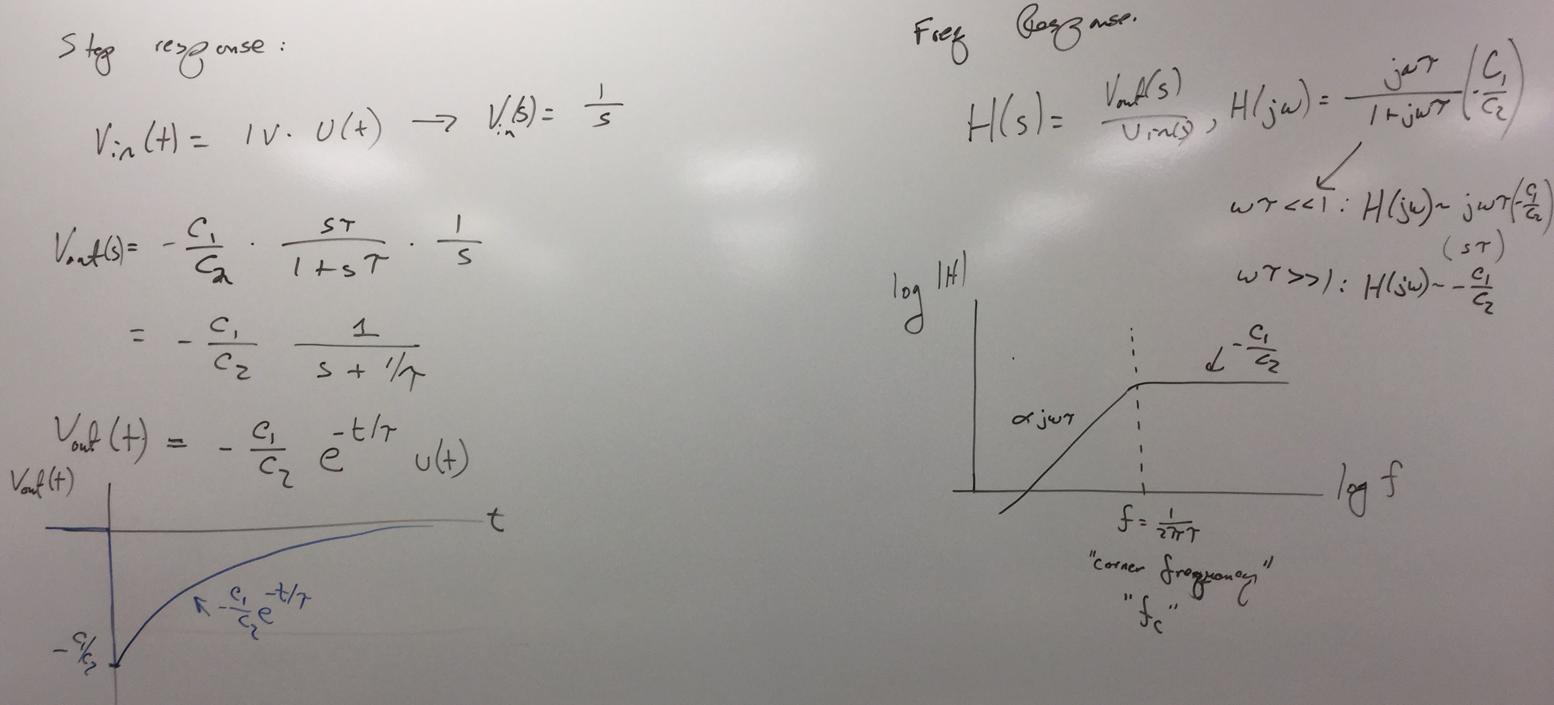
- Frequency response (Fig. 1):
Use your device function to do a frequency sweep.
the device inputs a single frequency and measures the result.
Compare your measured frequency response to your expected result.
- Change resistor, change capacitor value.
Both analytically predict the response and measure
the time-domain response and frequency response.
Compare the analytical values with the devices used.
You will want the step response results and time-constant results
efficiently plotted in your report.
You will want a single plot of the two frequency responses.
- From the components you have available, set up the circuit in Fig. 2 having a low-frequency gain
greater than 3 and a timeconstant within an order of magnitude of Fig. 1.
You should analyze this circuit for its step response and frequency response.
Perform a similar Step response , curve fit for timeconstant,
and Frequency response (one set of resistors)
for this circuit as you did for the circuit in Fig. 1.
- Tentitive Rubric for this project.
- A previous year
( Spring 2019 )
lab experiment and two good examples
(a and b)
of writeups to these experiments. I am not saying these writeups were perfect,
and yet they were good examples of the better writeups for that semester.
|